3 Diagnostic Tools for Cartridge Case Comparison Algorithms
Abstract
Forensic comparison algorithms are useful for measuring the probative value of a collection of evidence.
A number of algorithms pre-process, compare, and return some measure of similarity for two pieces of evidence.
Rarely, however, are there mechanisms built into the algorithm to indicate when a step goes awry.
For example, poorly-calibrated pre-processing of the evidence can have substantial impact on downstream results, which may lead to incorrect or misleading conclusions.
Even for well-calibrated algorithms, the resulting similarity measure can be difficult to justify or explain.
Diagnostics are useful as a supplementary tool for explaining the behavior of a complex model or algorithm.
In this paper, we introduce a suite of visual and interactive diagnostic tools to assess algorithms that automatically compare forensic cartridge case evidence.
These tools are useful to both forensic researchers and practitioners.
Researchers can analyze and correct the (mis)behavior of the algorithm while forensic practitioners can more easily understand and explain the algorithm.
We develop a collection of tools to diagnose each step of a cartridge case comparison algorithm and implement in in an R package called impressions.
We then implement these visual diagnostics in an interactive web application called cartridgeInvestigatR to also allow non-programmers to interact with and explore these algorithms.
We provide both the impressions package and cartridgeInvestigatR as free, open-source software.
3.2 Background and Introduction
Forensic examinations are intended to provide an objective assessment of the probative value of a piece of evidence. Typically, this assessment of probative value is performed by a forensic examiner who visually inspects the evidence to determine whether it matches evidence found on a suspect. The process by which an examiner arrives at their evidentiary conclusion is largely opaque and has been criticized (President’s Council of Advisors on Sci. & Tech. 2016) because its subjectivity does not allow for an estimation of error rates. In response, National Research Council (2009) pushed to augment subjective decisions made by forensic examiners with automatic, statistically-founded algorithms that objectively assess evidence and can be explained during court testimony. These algorithms enable the quantification of an examiner’s uncertainty by measuring the probative value of a piece of evidence.
A cartridge case (left of Figure 3.1) is the portion of firearm ammunition that encases a projectile (e.g., bullet, shots, or slug) along with the explosive used to propel the projectile through the firearm. When a firearm is discharged, the projectile is propelled down the barrel of the firearm, while the cartridge case is forced towards the back of the barrel. The base of the cartridge case (middle of Figure 3.1) strikes the back wall, known as the breech face, of the barrel with considerable force, thereby imprinting any markings on the breech face onto the cartridge case and creating the so-called breech face impressions (right of Figure 3.1). These markings have been suggested to be unique to a firearm and are used in forensic examinations to determine whether two cartridge cases have been fired by the same firearm.

Figure 3.1: (Left) Fired cartridge case and bullet, (Middle) Base of the cartridge case that comes into contact with the breech face of the firearm, (Right) Zoom into the primer region showing breech face impressions.
We measure the surface of a cartridge case using a TopMatch-3D High-Capacity Scanner by Cadre Forensics\(^{\text{TM}}\). This scanner collects images under various lighting conditions of a gel pad into which the cartridge case surface is impressed and combines these images into a regular 2D array called a surface matrix. Examples of two such surface matrices are shown in the middle of Figure 3.2. The physical dimensions of these objects are about 5.5 \(mm^2\) captured at a resolution of 1.84 microns per pixel (1000 microns equals 1 mm). Each element of the surface matrix corresponds to the height of the impressed gel at that location. The nominal resolution for height measurements depends on the viscosity of the gel and is reported to be better than 1 micron. The breech face impression regions have been manually annotated (in red). Using this manual annotation, we isolate the breech face impression region. Note that this introduces structurally missing values into the scan.
Figure 3.2 shows the isolated breech face impression regions where the height values of the surface have been mapped to a diverging purple (low) to orange (high) color scale and missing values are shown in gray.
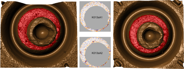
Figure 3.2: (Left) Cartridge case scan K013sA1 with breech face (BF) impressions manually annotated in red, (Middle) Processed surface matrices, (Right) Cartridge case scan K013sA2 with breech face (BF) impressions manually annotated in red. Raw scans (left and right) and processed versions of the surface matrices (in the middle) for a pair of cartridge cases fired by the same handgun (Ruger SR9, Gun A1, SerialNo 331-96383).
Even among matching cartridge case pairs, we have found results like those shown in Figure @ref(fig:cmcPlot_match), where only a small number of the total cells are classified as CMCs, to be quite common. An underlying assumption of the CMC methodology is that many source cells should find the “correct” registration in a matching target scan. However, it can be difficult to determine why a particular cell did or did not register correctly. In this paper, we introduce diagnostic tools that can be used to visually and numerically characterize the quality of alignment of cells. We also demonstrate how the numerical diagnostics can be used as features to classify matching and non-matching cartridge case pairs.
3.2.1 Notational Conventions
As the name implies, surface matrices are two-dimensional arrays whose elements contain relative height values of the corresponding cartridge case surface (“Geometrical product specifications (GPS) — Surface texture: Areal — Part 72: XML file format x3p” 2017). For notational simplicity, we assume that the matrices are square, i.e. \(A \in \mathbb{R}^{k \times k}\) for some matrix \(A\) and \(k > 0\). Note, that any assumption of sizing of matrices are easily enforced by padding with additional missing values. Due to the presence of (structural) missing values around the breech face impression, additional padding does not interfere with the structure of the scan. We use lowercase letters with subscripts to denote a particular value of a matrix; e.g., \(a_{ij}\) is the value in the \(i\)th row and \(j\)th column, starting from the top left corner, of \(A\).
For the purpose of dealing with missing values mathematically, we adapt standard matrix algebra as follows: if an element of either matrix \(A\) or \(B\) is missing, then any element-wise operation including this element is also missing, otherwise standard matrix algebra holds. For example, for matrices \(A\) and \(B \in \mathbb{R}^{k \times k}\) we define the addition operator as: \[ A \oplus_{\tiny{NA}} B = \left( a_{ij} \oplus_{\tiny{NA}} b_{ij} \right)_{1 \le i,j \le k} := \begin{cases} a_{ij} + b_{ij} & \text{ if both } a_{ij} \text{ and } b_{ij} \text{ are numbers}\\ \text{NA } & \text{ otherwise} \end{cases} \] Operations \(\ominus_{\tiny{NA}}\) as well as all comparisons are defined similarly. For the purpose of readability, we will use the standard algebraic operators \(+, -, >, <, ...\) and apply the extended operations as defined above.
3.2.2 Registration Procedure
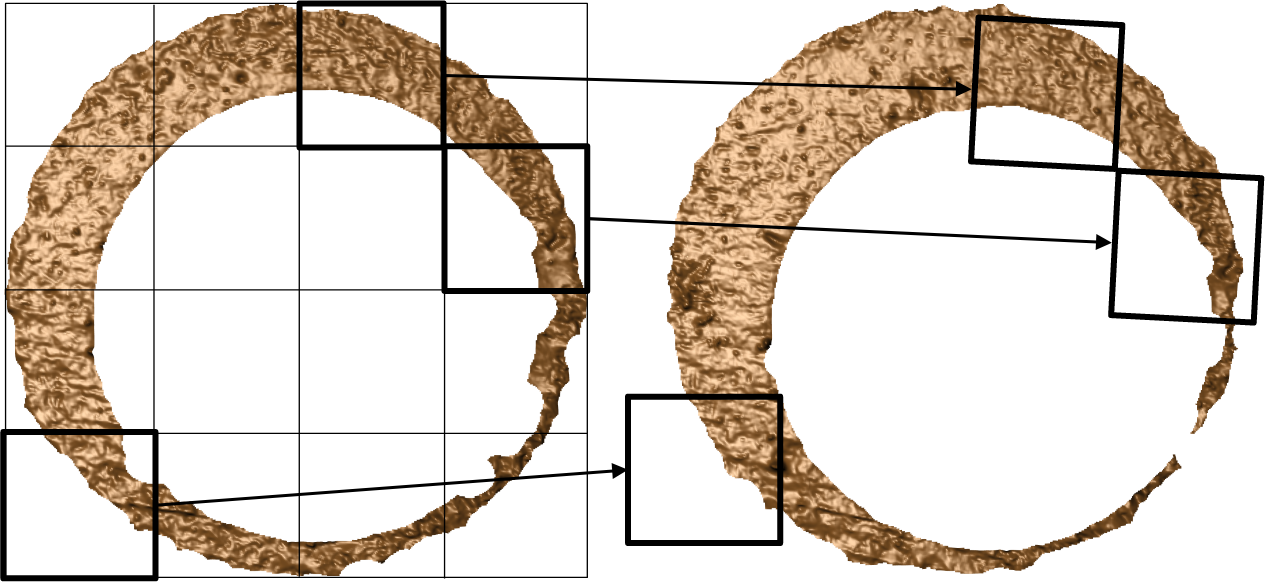
Figure 3.3: The process of “registering” a surface matrix to another involves determining the rotation and translation that optimally aligns the two surfaces. We can perform this registration both at the full scan and cell-based (which is illustrated above) scales. In the visualization, we show how three cells in the scan on the left register in the scan on the right.
A critical step in comparing \(A\) and \(B\) is to find a transformation of \(B\) such that it aligns best to \(A\) (or vice versa). In image processing, this is called image registration. Noting that \(A\) and \(B\) are essentially grayscale images, we rely on a standard image registration technique (Brown 1992).
In our application, a registration is composed of a discrete translation by \((m,n) \in \mathbb{Z}^2\) and rotation by \(\theta \in [-180^\circ,180^\circ]\). To determine the optimal registration, we calculate the cross-correlation function (CCF) between \(A\) and \(B\), which measures the similarity between \(A\) and \(B\) for every possible translation of \(B\), denoted \((A \star B)\). We estimate the registration by calculating the maximum CCF value across a range of rotations of matrix \(B\). Let \(B_\theta\) denote \(B\) rotated by an angle \(\theta \in [-180^\circ,180^\circ]\) and \(b_{\theta_{mn}}\) the \(m,n\)-th element of \(B_\theta\). Then the estimated registration \((m^*,n^*,\theta^*)\) is:
\[ (m^*,n^*,\theta^*) = \arg \max_{m,n,\theta} (a \star b_\theta)_{mn}. \]
In practice we consider a discrete grid of rotations \(\pmb{\Theta} \subset [-180^\circ,180^\circ]\). The registration procedure is outlined in the image registration algorithm. We refer to the matrix that is rotated as the “target.” The result is the estimated registration of the target matrix to the “reference” matrix.
Image Registration Algorithm
We can apply the image registration in both directions to align not only scan \(B\) to \(A\), but also \(A\) to \(B\). Theoretically, these two registrations should be exact opposites of each other. However, depending on the scans this may not happen in practice because we use “nearest-neighbor” interpolation to rotate the discretely-indexed surface matrices. To accommodate these two comparison directions, we now introduce a subscript \(d = A,B\) that refers to the source scan used in the image registration. For example, \((m_A^*, n_A^*, \theta_A^*, CCF_{\max,A})\) refers to the estimated registration and CCF from aligning scan \(B\) to \(A\).
Song (2013) points out that two matching cartridge cases may only have a handful of regions with distinguishable, matching impressions due to inherent variability in the firing process. Calculating a correlation between two full scans as in image registration algorithm may not highlight their similarities. Instead, Song (2013) proposes partitioning one of the scans into a grid of “cells” and estimating the registration between each cell and the other scan.
We now extend the surface matrix notation introduced previously to accommodate cells. Let \(A_{t}\) denote the \(t\)th cell of matrix \(A\), \(t = 1,...,T_A\) where \(T_A\) is the total number of cells containing non-missing values in scan \(A\) and let \((a_t)_{ij}\) denote the \(i,j\)-th element of \(A_t\). This procedure can be viewed as a generalization of image registration algorithm that we call the “cell-based comparison procedure” and outlined below.
Cell-Based Comparison Algorithm
The output of the cell-based comparison is a set of estimated registrations - one registration for each cell in the source scan for each \(\theta\). For a particular cell \(t \in \{1,...,T_A\}\), we select the registration that maximizes the CCF across all \(\theta \in \pmb{\Theta}_A'\) as its estimated registration.
Similar to image registration algorithm, we can use cell-based comparison to align not only cells from \(A\) to \(B^*\), but also cells from \(B\) to \(A^*\), which is an aligned version of scan \(A\) from image registration algorithm using \(B\) as source. We again use a direction subscript \(d = A,B\) to refer to the source scan in cell-based comparison. For example, the outcome of cell-based comparison using \(B\) as source and \(A^*\) as target is the set \(\pmb{F}_B\) of estimated registrations per cell, \(t = 1,...,T_B\), per rotation, \(\theta \in \pmb{\Theta}_B'\).
A consequence of the scanning process is that the physical location of any measured values is relative, but the relationship of the measurements to each other is fixed. This means that we can, without affecting any structure in a scan, translate and even rotate measurements in 3d space. For the purpose of making scans comparable to each other during registration, we subtract the mean surface depth value from each scan, making the mean surface value effectively 0. This is commonly performed when computing the cross-correlation function in image registration applications.
One challenge with using registration algorithms, such as the image registration and cell-based comparison procedures ,is understanding when and how they “work” as expected. For example, we expect for truly matching cartridge cases that these estimated registrations should “agree” across various cells. In other words, that \((m^*_{A,t,\theta},n^*_{A,t,\theta}, \theta)\) should be the same for all \(t = 1,...T_A\). We don’t assume such agreement will occur for truly non-matching cartridge cases. Rarely do all cells agree with the same registration in practice, even for truly matching cartridge cases. Instead, depending on the quality of the impressions on two matching cartridge cases, there may be a handful of cells that have similar \((m^*_{A,t,\theta},n^*_{A,t,\theta}, \theta)\) values. A natural question is: why do some scans/cells find the correct registration while others do not? In the next section, we introduce a set of diagnostic tools we developed to answer such questions.
3.3 Visual Diagnostics
3.3.1 The X3P Plot
The first visual diagnostic tool we discuss is the “X3P plot” which is used to visualize the values of a scan’s surface matrix. We show an example of an X3P plot in Figure 3.5, which will be discussed in more detail below. The orientation of the X3P plot is the same as its underlying surface matrix, meaning the top left-most pixel represents the \([1,1]\)-th element of the surface matrix followed the \([1,2]\)-th element to its immediate right and so on. To construct the X3P plot, we map 11 percentiles of the non-missing values in a surface matrix to the continuous, divergent purple-white-orange color scheme illustrated in Figure 3.4. The darkest shades of purple and orange represent the minimum and maximum surface values, respectively. We use a very light shade of gray to represent the median surface value to ensure symmetry in the percentile mapping. Rather than mapping deciles to the 11 colors (minimum, 10th percentile, 20th percentile, etc.), we’ve found the more polarized mapping shown in Figure 3.4 to be more effective at emphasizing extreme surface values, which are commonly associated with the most prominent impressions.

Figure 3.4: The percentiles (top) and hexidecimal color values (bottom) used in the color mapping of the X3P plot.
To visualize two or more scans using the X3P plot, we map percentiles of the pooled surface values to the same color scale. This allows us to compare the relative sizes of impressions across multiple cartridge cases. The registration procedure outlined in the image registration algorithm is highly sensitive to extreme values on either surface, so performing a visual comparison of two scans using the X3P plot is useful for identifying whether further processing of either scan is needed.
Figure 3.5 shows two examples of the registration output for a matching pair of scans labeled K002eG2 and K227iG3. In the top plot we see that both scans contain large, extraneous markings that may affect the registration procedure. There is a ring of raised observations around the center of K002eG2 that is an artifact of the deformation that occurs when the firing pin strikes the cartridge case primer. Additionally, there are large dent-like markings on both K002eG2 and K227iG3. Registering these two scans using the image registration algorithm results in \(CCF_{\max} = 0.14\) at registration \((m^*,n^*,\theta^*) = (4,19,-6^\circ)\).
The bottom plot of Figure 3.5 shows the registrations of K002eG2 and K227iG3 after applying the additional pre-processing of removing the extraneous regions. The output of the image registration algorithm is now \(CCF_{\max} = 0.29\) at registration \((m^*,n^*,\theta^*) = (6,18,-6^\circ)\). Although the registrations are similar for both pairs of scans, the cross-correlation value more than doubles when we remove the extraneous regions. We also note that removal of the extreme values makes it easier to visually identify similar markings between K002eG2 and K227iG3, such as the “striped” impressions at the top of the two scans. Highlighting such similarities is one of the strengths of the X3P plot.
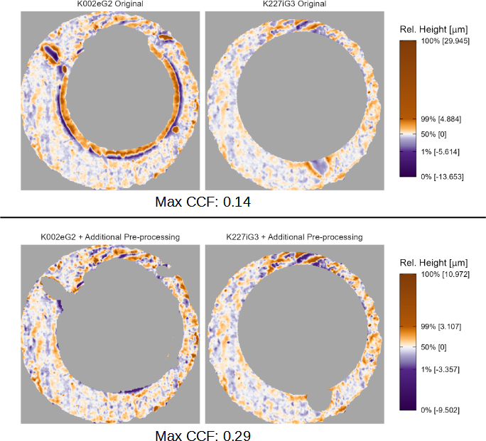
Figure 3.5: Registration results from comparing two versions of a matching pair of cartridge case scans. In the first comparison (top), extraneous values are left in the scan which causes the overall \(CCF_{\max}\) value to be relatively low (0.14). When these values are removed (bottom), the CCF value more than doubles to 0.29. The X3P plot is useful for identifying scans that are in need of additional pre-processing.
3.3.2 The Comparison Plot
The “comparison plot” is a visual diagnostic tool that uses the X3P plot to directly compare the surface values of two scans. The comparison plot provides a quick, intuitive assessment by partitioning the surfaces into similarities and differences. To construct the comparison plot we first obtain two aligned scans \(A\) and \(B^*\) using the image registration algorithm. A comparison plot like the one shown in Figure 3.8 depicts aligned versions of the two scans \(A\) = K013sA1 and \(B\) = K013sA2 shown in Figure 3.2. The first columns shows the scan \(A\) and aligned scan \(B^*\) in the top left and right, respectively. The dark gray (gray40) elements in these two visualizations represent the non-overlapping elements from the other scan. Next, we wish to partition these \(A\) and \(B^*\) into similarities and differences using a filter operation.
For a matrix \(X \in \mathbb{R}^{k \times k}\) and Boolean-valued condition matrix \(cond: \mathbb{R}^{k \times k} \to \{TRUE,FALSE\}^{k \times k}\), we define an element-wise filter operation \(\mathcal{F}: \mathbb{R}^{k \times k} \to \mathbb{R}^{k \times k}\) as:
\[\begin{align*} \mathcal{F}_{cond}(X) = (f_{ij})_{1 \leq i,j \leq k} = \begin{cases} x_{ij} &\text{if $cond$ is $TRUE$ for element $i,j$} \\ NA &\text{otherwise.} \end{cases} \end{align*}\]
The resulting \(\mathcal{F}_{cond}(X)\) is a copy of the matrix \(X\) where elements for which \(cond\) is \(TRUE\) are replaced with \(NA\). The filtering operation allows us to isolate elements of a surface matrix that satisfy some criterion. For example, we can isolate a surface matrix to only those elements that are close to the elements of another surface matrix.
Figure 3.6 shows the construction of a filtered element-wise average between \(A\) and \(B^*\). We compute the element-wise average \(\frac{1}{2}(A + B^*)\) and absolute difference \(|A - B^*|\) as shown in the left and right of Figure 3.6. We then consider values of \(|A - B^*|\) that are greater than some threshold \(\tau > 0\). We construct Boolean-valued matrices \(|A - B^*| \leq \tau\) and \(|A - B^*| > \tau\) based on whether the element-wise absolute difference is at most or greater than \(\tau\). For example, the right side of Figure 3.6 shows the elements of matrix \(|A - B^*| \leq 1\) with \(TRUE\) elements represented as white pixels and \(FALSE\) elements as black pixels. We then filter \(\frac{1}{2}(A + B^*)\) using \(|A - B^*| \leq \tau\) as the \(cond\) matrix, resulting in tge filtered element-wise average \(\mathcal{F}_{|A - B^*| \leq \tau}\left(\frac{1}{2}(A + B^*)\right)\), an example of which is shown at in the bottom of Figure 3.6 using \(\tau = 1\).
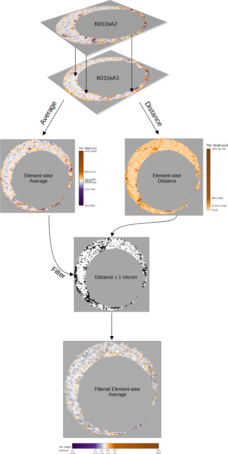
Figure 3.6: To construct the comparison plot after aligning the scans K013sA1 and K013sA2, we compute their element-wise average (left) and element-wise absolute difference (right). We then compute a Boolean-valued matrix based on whether the elements of the element-wise absolute difference is greater or less than 1 micron (right). We use this Boolean matrix to distinguish between similarities and differences in the scan impressions.
Complementary to the filtered element-wise average, the right column of the comparison plot shows differences between the two scans. While it is visually obvious when scans share similar markings, characterizing different markings can be challenging. For example, two markings may be different in their depth, shape, orientation, or spatial relationship to other markings. As such, we visualize two filtered versions of the aligned scans \(\mathcal{F}_{|A - B^*| > \tau}(A)\) and \(\mathcal{F}_{|A - B^*| > \tau}(B^*)\) to emphasize differences. Figure 3.7 shows an example of the results of this filtering using \(\tau = 1\).
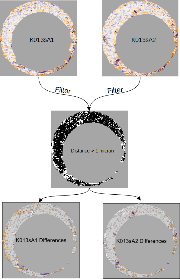
Figure 3.7: To construct the comparison plot, we filter two scans \(K013sA1\) and \(K013sA2\) based on regions where their element-wise absolute difference exceeds 1 micron, which are represented as white pixels in the black and white image. This emphasizes regions where the two surfaces differ, which complements the similarities that are emphasized in the element-wise average.
The comparison plot visualizes the surface values of the original scans \(A\) and \(B^*\), the filtered element-wise average \(\mathcal{F}_{|A - B^*| \leq \tau}\left(\frac{1}{2}(A + B^*)\right)\), and filtered element-wise differences \(\mathcal{F}_{|A - B^*| > \tau}(A)\) and \(\mathcal{F}_{|A - B^*| > \tau}(B^*)\). Figure 3.8 shows an example of a comparison plot using \(A=\) K013sA1 and \(B=\) K013sA2.
The middle column of the comparison plot shows the filtered element-wise matrix \(\mathcal{F}_{|A - B^*| \leq \tau}\left(\frac{1}{2}(A + B^*)\right)\). By isolating the element-wise average to “close” surface values between \(A\) and \(B^*\), the filtered element-wise average emphasizes similar markings between the two scans. In Figure 3.8, we use a filtering threshold of \(\tau = 1\) microns and represent filtered elements in light gray (gray80). This filtered element-wise average illustrates that there are many similarities between the two surfaces. To identify similarities using the element-wise average, we have found it most effective to scan the filtered element-wise average plot for distinctive markings, such as the deep purple and orange markings in the 5 o’clock position of the firing pin hole in Figure 3.8. After identifying distinctive markings, it is relatively easy to identify the contributing markings from \(A\) and \(B^*\) by considering the same region in the two plots in the left column. For example, we see deep purple and orange striped impressions in the 5 o’clock positions of \(A\) and \(B^*\) in Figure 3.8. Cross-referencing the filtered element-wise average with the individual scans allows us to assess the degree of similarity and spatial relationship between markings on the two scans.
The right column of Figure 3.8 shows the filtered differences between scans \(A\) and \(B^*\) using a cutoff threshold of \(\tau = 1\) microns. Again, we’ve found it useful to study the two filtered plots to identify differences that can be cross-referenced against the original scans. For example, scan \(B^*\) has a dent-like marking at the 11 o’clock position of the firing pin hole that is not present in \(A\). On the other hand, we note a dark orange region in the 5 o’clock position, where we had previously noted similarities, that is treated as a difference. Considering the original scans in the left column, we see that these orange regions are indeed part of the striped purple and orange impression region. It can be safely assumed that these two regions should be treated as “similar” markings despite being at least 1 micron apart. These two examples illustrate the fundamental challenge with characterizing differences - there are many ways in which two markings can be “different” from one another.
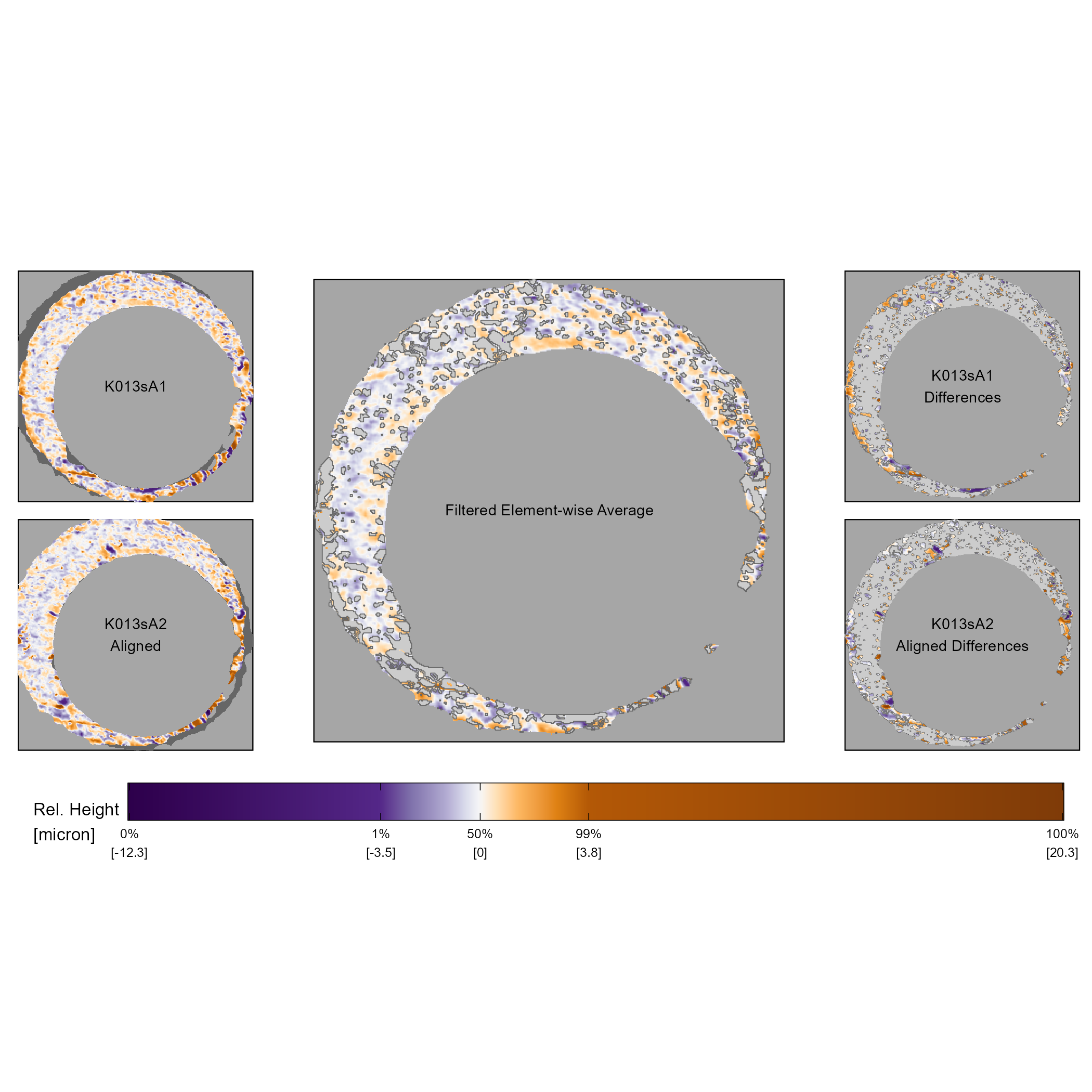
Figure 3.8: The comparison plot provides an intuitive visualization of the similarities and differences between two aligned surface matrices. The left column of the comparison plot shows two aligned scans. The middle column shows the element-wise average between the two aligned scans after filtering out surface values that are at least 1 micron apart. The right column shows these filtered surface values of the aligned scans. Together, the middle and right column show the “similarities” and “differences” between the two aligned scans.
By construction, the X3P and comparison plots emphasize the most extreme values in the two surface matrices. This means that similar, yet less extreme markings are harder to visually identify using the full scan X3P and comparison plots. To visually assess the similarity between these markings, we can “zoom in” to specific regions of the cartridge case surfaces using the cell-based comparison procedure outlined in the cell-based comparison procedure. Recall that the cell-based comparison returns a set of estimated registrations, one for each source cell \(t = 1,...,T_A\). Using these estimated registrations, we extract a matrix from the target scan that represents the patch in the target scan that maximized the CCF with the source cell. That is, we extract the target “mate” for each source cell. Figure 3.9 shows the comparison plot of cell 3, 8 from scan K013sA1 and its target mate in K013sA2. The left column again shows the two aligned surface matrices, the middle column the filtered element-wise average using \(\tau = 1\) microns, and the right column the filtered differences. Compared to the depiction of this region in Figure 3.8, it is much easier to identify similar and different markings using this zoomed-in visualization. For example, the dark purple “dots” on the upper-left side of the two scans are more prominent in this visualization. We note that the color scale mapping now ranges from -5 to 4.1 microns compared to -12.3 to 20.3 microns in Figure 3.8. Small, local markings are more prominent when we use the comparison plot on the output of the cell-based comparison procedure.
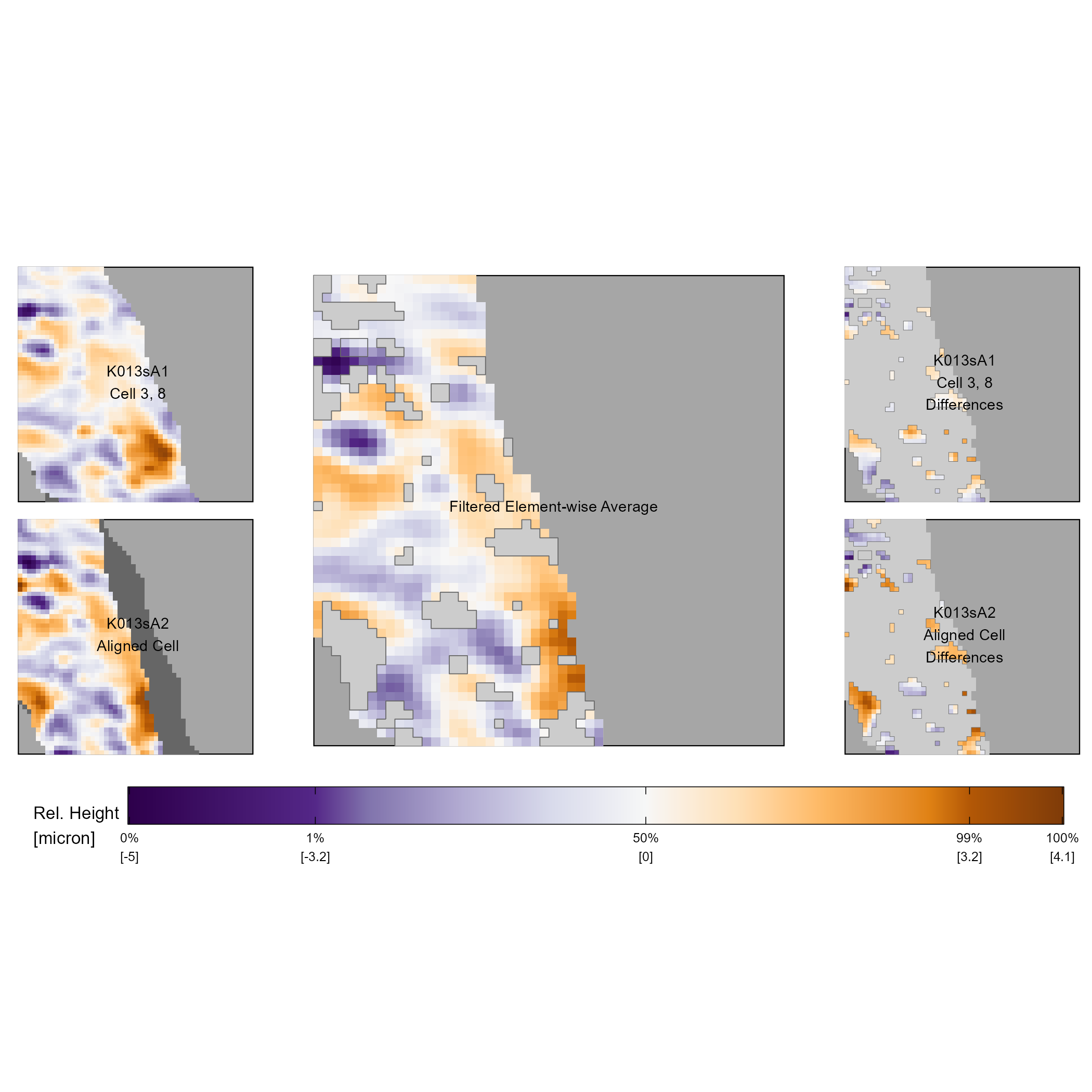
Figure 3.9: The comparison plot for cell 3, 8 of scan K013sA1 and its aligned mate in scan K013sA2. The left column shows the surface values of these two cells. Note that non-overlapping pixels are shown in dark gray in the bottom left plot. The middle column shows similarities between the surfaces in the form of the filtered element-wise average. The right column shows the surface values with the opposite filtering used in the filtered element-wise average plot. We use a gray border to emphasize the filtered vs. non-filtered regions.
The comparison plot is particularly useful for understanding the results of the cell-based registration procedure outlined in the cell-based comparison. For example, the top of Figure 3.10 shows an aligned cell 6, 1 between two non-match scans K013sA1 and K002eG1. It’s difficult to visually identify many similarities between the two scans, which is expected given that the cartridge cases originate from different firearms. However, the bottom of Figure 3.10 depicting the comparison plot between the aligned cell 6, 1 pair demonstrates that there are actually local similarities. From the element-wise average we see that there are similar purple and orange regions shared between these two cells.
This example underscores the need to analyze both similarities and differences when comparing two scans. We’re bound to find similarities if this is all we look for, so we also need to describe the differences between the surfaces. In the next section, we discuss a set of summary statistics computed from the Comparison Plot that quantify both the similarities and differences between two scans.
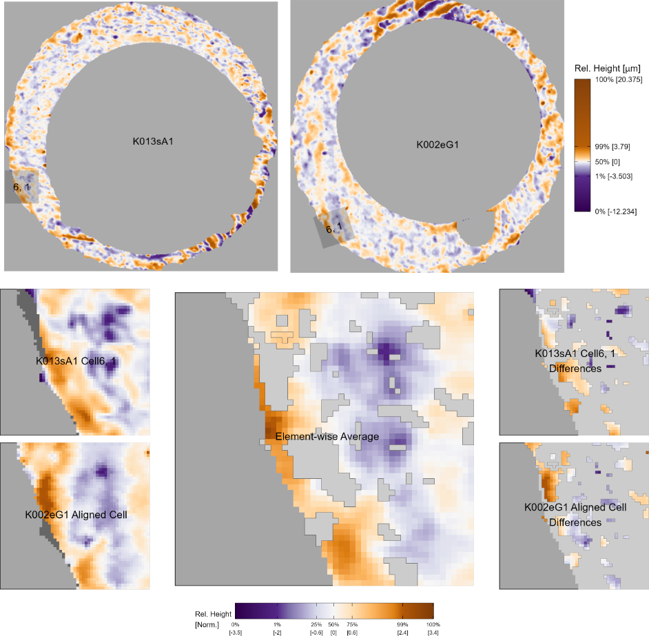
Figure 3.10: (Top) We consider a non-match pair of cartridge cases K013sA1 and K002eG1 that don’t appear to share many similar markings at first glance. (Bottom) After registering cell 6, 1 from K013sA1 in K002eG1 using the cell-based comparison, we then consider the Comparison Plot between the aligned pair of cells. Using this zoomed-in view, we can clearly see that there are actually local similarities between the two cartridge cases despite being fired from different firearms. This demonstrates how the comparison plot is useful for understanding registration results from cell-based comparison.
3.3.3 Visual Diagnostic Statistics
In the last section, we used the comparison plot to make a number of qualitative observations about the similarities and differences between the impressions of two pairs of cartridge cases. These observations aligned with what our intuition says should be true for two matching/non-matching cartridge cases. For example, we would expect there to be many more similarities than differences for a matching pair compared to a non-matching pair. In this section, we translate these sorts of qualitative observations into a set of numerical features that can be used to determine whether two cartridge case scans were fired from the same firearm.
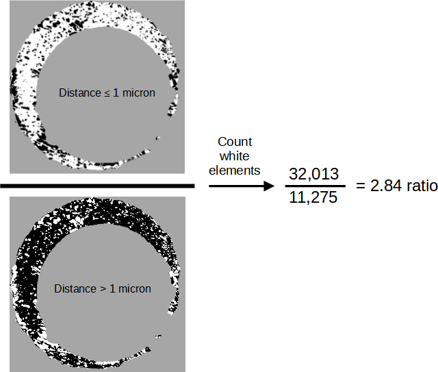
Figure 3.11: We compute the ratio between the number of similar and different elements of two aligned scans, which are defined to be elements for which the two surfaces are at most or greater than 1 micron, respectively. These are represented above as white pixels in the two images on the left. We then count the number of white pixels in each image and compute their ratio, resulting in this example in a value of 2.84. We expect this ratio to be larger for matching comparisons, on average, than non-matching comparisons.
The first statistic is the ratio between the number of similarities and differences for a pair of scans. To compute this, we consider the number of \(TRUE\) elements the \(cond\) matrices \(|A - B^*| \leq \tau\) and \(|A - B^*| > \tau\). Figure 3.11 shows an example of this ratio computed for the matching pair K013sA1 and K013sA2, which results in a value of 2.84 meaning there are almost three times as many similarities as there are differences between the two scans.
Mathematically, the similarities vs. differences ratio is given by
\[\begin{equation} r_{d} = \frac{\pmb{1}^T I(|A - B^*| \leq \tau) \pmb{1}}{\pmb{1}^T I(|A - B^*| > \tau) \pmb{1}} \tag{3.1} \end{equation}\]
where \(\pmb{1} \in \mathbb{R}^k\) is a column vector of ones and \(I(\cdot)\) is the element-wise, matrix-valued indicator function. The inner products in the numerator and denominator act to count the number of TRUE elements in the two complementary \(cond\) matrices.
We also compute similarities vs. differences ratios for the results of the cell-based comparison procedure outlined in cell-based comparison. Specifically, we compute the ratio for a cell from the source matrix and its aligned mate in the target matrix, resulting in the ratio value \(r_{d,t}\). We expect that the similarities vs. differences ratio will be larger for matching comparisons compared to non-matching comparisons.
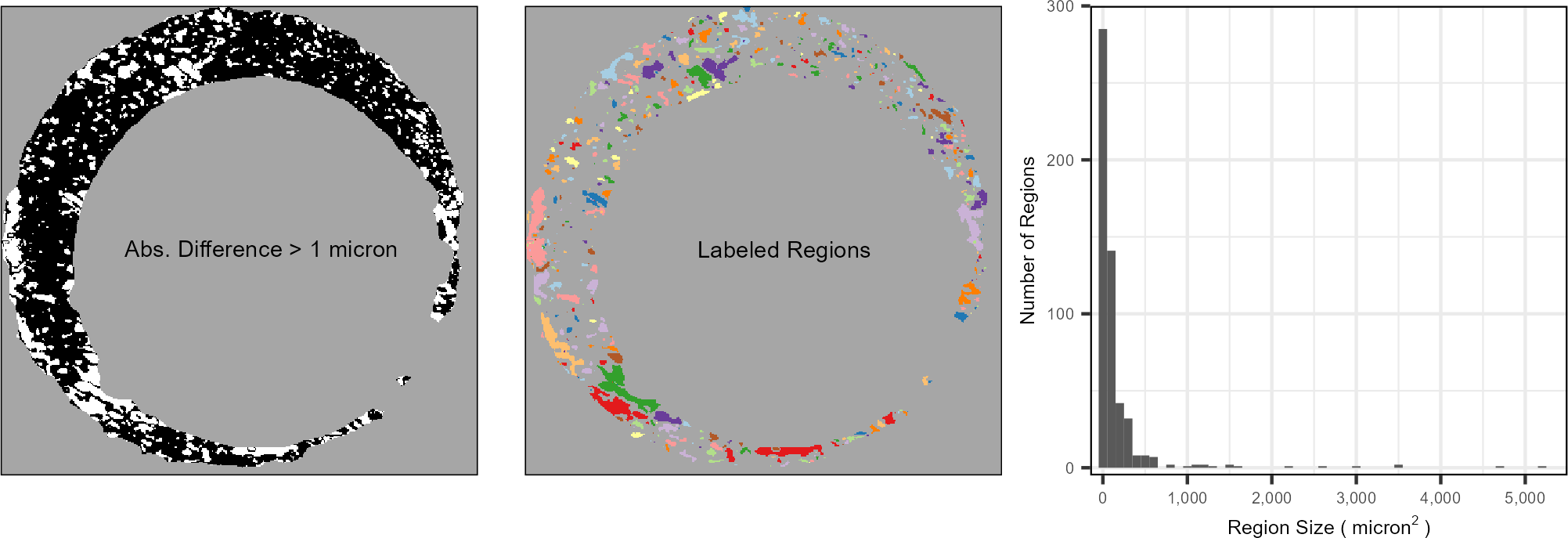
Figure 3.12: (Left) After aligning two scans, we filter regions that are “different” from each other, meaning the absolute difference between surface values is larger than some threshold. We binarize the scan into different vs. similar regions - shown in white and black, respectively. (Middle) Using a connected components labeling algorithm, we identify connected “neighborhoods” of filtered elements, which are distinguished here by fill color. (Right) Considering the distribution of the region sizes, we see that the vast majority of the regions are relatively small, under 1000 square microns, although there are some outliers. We assume that the average region size will be relatively small for truly matching comparisons.
We assume markings on the surfaces of two aligned, matching cartridge cases will line up with each other. This implies that regions that we define as “different” should be relatively small in area. We translate this into a numerical feature by considering the \(TRUE\) elements of the \(cond\) matrix \(|A - B^*| > \tau\), which are elements where the surfaces differ by at least \(\tau\). For example, the left side of Figure 3.12 shows the matrix \(|A - B^*| > 1\) for \(A\) = K013sA1 and \(B\) = K013sA2 with \(TRUE\) elements represented in white. We then use a connected components labeling algorithm detailed in Hesselink, Meijster, and Bron (2001) and implemented in Barthelme (2019) to identify connected “neighborhoods” of \(TRUE\) elements. Specifically, the algorithm returns a set of sets \(\pmb{S}_d = \{S_{d,1},S_{d,2},...,S_{d,L_d}\}\) where each \(S_{d,l}\) is a set of indices of the \(cond\) matrix that have a value of \(TRUE\) and are connected by a chained-together sequence of 4 (Rook’s) neighborhoods. The middle of Figure 3.12 shows each \(S_{d,l}\) distinguished by different fill colors, \(l = 1,...,L_d\).
The right side of Figure 3.12 shows a histogram of the region sizes, denoted \(|S_{d,l}|\) for \(l = 1,...,L_d\). We see that most of the sizes are relatively small, which agrees with our initial assumption. There are a handful of larger regions that, when cross-referenced with the surface values in the original scans (see Figure 3.8, for example), are clearly different from each other, meaning the visual diagnostic works as intended. We assume that the distribution of region sizes for a matching pair will have far fewer extreme values compared to a non-matching pair. Again, we extend our notation to accommodate individual cells. Let \(\pmb{S}_{d,t} = \{S_{d,t,1},...,S_{d,t,L_{d,t}}\}\) denote the set of labeled neighborhoods for a cell \(t = 1,...,T_d\), \(d = A,B\).

Figure 3.13: The plots show regions of two aligned cells from a matching comparison. Specifically, we filter these cells to only elements for which the surfaces are at least 1 micron apart. We note here that even among these “different” regions, the trends in the surface values are similar, which may occur because of inconsistent contact with markings on the breech face of a firearm across repeated fires. The relatively high correlation between these two cells of 0.84 reflects this similarity.
The final statistic we compute is based on the observation that, even among regions that we define as “different,” the surface values of two matching cartridge cases should follow similar trends. There may be variability in the depth of markings impressed by a firearm’s breech face across repeated fires, but the overall shape/trend of the markings should remain consistent. For example, Figure 3.13 shows regions of two cells from a comparison between matching scans \(A\) = K013sA1 and \(B\) = K013sA2. We filter these two cells to elements where their surfaces are at least one micron apart. The surface values of these “differences” vary in a similar manner despite being far from each other. This observation is represented in the correlation value 0.84, which is relatively high for cartridge case comparisons. We calculate the correlation by vectorizing the two filtered surface matrices and treating missing values by case-wise deletion.
To measure the similarity in the surface value trends, we calculate the correlation \(cor_{d,\text{full},\text{diff}}\) between the filtered matrices \(\mathcal{F}_{|A - B^*| > \tau}(A)\) and \(\mathcal{F}_{|A - B^*| > \tau}(B^*)\) for \(d = A\) and \(\mathcal{F}_{|A^* - B| > \tau}(A^*)\) and \(\mathcal{F}_{|A^* - B| > \tau}(B)\) for \(d = B\). We assume that \(cor_{d,\text{full},\text{diff}}\) will be large for matching cartridge case pairs relative to non-matching pairs. Said another way, we assume that regions of matching cartridge cases that are different will still follow similar trends. This can occur due to variability in the amount of contact between a cartridge case and breech face across multiple fires of a single firearm.
We extend our notation to accommodate cell comparisons \(t = 1,...,T_d\) for \(d = A,B\) using subscripts: \(cor_{d,t,\text{diff}}\). For example, \(cor_{A,t,\text{diff}}\) is the correlation between cell filtered surface matrices \(\mathcal{F}_{|A_t - B_{t,\theta_t^*}^*| > \tau}(A_t)\) and \(\mathcal{F}_{|A_t - B_{t,\theta_t^*}^*| > \tau}(B_{t,\theta_t^*}^*)\) where \(B_{t,\theta_t^*}^*\) is the matrix extracted from \(B^*\) that maximizes the CCF with \(A_t\). Figure 3.13 shows an example of computing the correlation between cell 2, 8 from scan K013sA1 and its mate in K013sA2.
These visual diagnostic statistics provide a quantitative complement to the qualitative observations we draw from the Comparison Plot. They are useful by themselves to understand or justify why a source scan or cell aligned to a specific region in the target. In the next section, we explore their use as numerical features to distinguish between matching and non-matching comparisons.
3.4 Statistical Learning from Visual Diagnostics
In this section, we explore using the visual diagnostic statistics discussed above as features in a statistical classifier model to differentiate between matching and non-matching comparisons. We consider a data set of 210 cartridge cases scanned at the Roy J. Carver High Resolution Microscopy Facility at Iowa State University that were collected as part of a study by (Baldwin et al. 2014). The researchers fired the Remington 9mm centerfire cartridge cases from 10 Ruger SR9 pistols. We scanned these cartridge cartridge cases using the Cadre\(^{\text{TM}}\) 3D-TopMatch High Capacity Scanner. See Chapter 4 for more information on these cartridge case data.
3.4.1 Visual Diagnostic Statistics as Features
Let \(A\) and \(B\) denote cartridge case scans. We first perform the registration procedure of image registration algorithm in both comparison directions using a rotation grid of \(\pmb{\Theta} = \{-30^{\circ} , -27^{\circ}, ..., 27^{\circ}, 30^{\circ}\}\), resulting in estimated full scan registrations \((m_{A}^*, n_{A}^*, \theta_A^*, CCF_{\max,A})\) and \((m_{B}^*, n_{B}^*, \theta_B^*, CCF_{\max,B})\). Using these registrations, we obtain the aligned versions of the target scans; \(B^*\) for \(d = A\) and \(A^*\) for \(d = B\).
Next, we perform the cell-based comparison procedure of cell-based comparison using rotation grids \(\pmb{\Theta}_d' = \{\theta_d^* - 2^{\circ}, \theta_d^* - 1^{\circ},\theta_d^*,\theta_d^* + 1^{\circ}, \theta_d^* + 2^{\circ}\}\) for \(d = A,B\) in both comparison directions, resulting in cell-wise registration sets \(\pmb{F}_A\) and \(\pmb{F}_B\). For each cell \(t = 1,...,T_d\), we compute its estimated registration as:
\[\begin{align*} \theta_{d,t}^* &= \arg \max_\theta \{CCF_{\max, d, t, \theta} : \theta \in \pmb{\Theta}_d' \} \\ m_{d,t}^* &= m_{d,t,\theta_{d,t}^*}^* \\ n_{d,t}^* &= n_{d,t,\theta_{d,t}^*}^*. \end{align*}\]
Using this estimated registration, we extract the cell’s mate from the target scan. For \(d = A\) and some cell \(t\), let \(B_{t,\theta_{d,t}^*}^*\) denote its aligned mate in scan \(B^*\) and assume the converse for \(d = B\).
At this point, we have the aligned mates for the source scans in both comparison directions at two both the full scan and cell scales. Following the notion that many cartridge cases may only have a few areas with distinguishable markings, we expect the features at these scales to give us qualitatively different information. Features at the cell scale may help illuminate regions of high similarity between two scans that the full scan features are unable to discern. However, we’ve seen in the example of Figure 3.10 that even non-matching scans can share local similarities, in which case full scan features would prove more useful.
We consider the average full-scan similarities vs. differences ratio across the two comparison directions:
\[\begin{align*} r_{\text{full}} = \frac{1}{2}(r_A + r_B). \end{align*}\]
We expect \(r_{\text{full}}\) to be large for matching pairs compared to non-matching pairs. That is, truly matching pairs will have more similarities than differences.
We also calculate features based on the ratio for cell comparisons \(t = 1,...,T_d\), \(d = A,B\). Let \(r_{d,t}\) denote the ratio for cell comparison \(t\) in direction \(d\). We consider the average and standard deviation of the cell-based similarities vs. differences ratio:
\[\begin{align*} \bar{r}_{\text{cell}} &= \frac{1}{T_A + T_B} \sum_{d \in \{A,B\}} \sum_{t = 1}^{T_d} r_{d,t} \\ s_{\text{cell}, r} &= \sqrt{\frac{1}{T_A + T_B - 1} \sum_{d \in \{A,B\}} \sum_{t = 1}^{T_d} (r_{d,t} - \bar{r}_{\text{cell}})^2}. \end{align*}\]
We expect \(\bar{r}_{\text{cell}}\) and \(s_{\text{cell}, r}\) to be large for matching cartridge case pairs relative to non-match pairs.
We calculate the following features using the full-scan labeled neighborhoods:
\[\begin{align*} \overline{|S|}_{\text{full}} &= \frac{1}{L_A + L_B} \sum_{d \in \{A,B\}} \sum_{l=1}^{L_d} |S_{d,l}| \\ s_{\text{full},|S|} &= \sqrt{\frac{1}{L_A + L_B - 1} \sum_{d \in \{A,B\}} \sum_{l=1}^{L_d} (|S_{d,l}| - \overline{|S|}_{\text{full}})^2}. \end{align*}\]
We assume that the average and standard deviation of the full-scan neighborhood sizes will be small for matching cartridge case pairs relative to non-matching pairs. That is, we assume that the the regions of \(A\) and \(B\) that are different will all be small, on average, and vary little in size. This assumption is appropriate assuming that the breech face leaves consistent markings on fired cartridge cases.
We calculate the per-cell average and standard deviation of the labeled neighborhood cell size:
\[\begin{align*} \overline{|S|}_{d,t} &= \frac{1}{L_{d,t}} \sum_{l=1}^L |S_{d,t,l}| \\ s_{d,t,|S|} &= \sqrt{\frac{1}{L_{d,t} - 1} \sum_{l=1}^{L_{d,t}} (|S_{d,t,l}| - \overline{|S|}_{\text{cell},d,t})^2}. \end{align*}\]
We assume that the cell-based \(\overline{|S|}_{d,t}\) and \(s_{d,t,|S|}\) will be small, on average, for truly matching cartridge cases. Consequently, we use the sample average of these as features:
\[\begin{align*} \overline{|S|}_{\text{cell}} &= \frac{1}{T_A + T_B} \sum_{d \in \{A,B\}} \sum_{t=1}^{T_d} \overline{|S|}_{d,t} \\ \bar{s}_{\text{cell},|S|} &= \frac{1}{T_A + T_B} \sum_{d \in \{A,B\}} \sum_{t=1}^{T_d} s_{d,t,|S|}. \end{align*}\]
We assume that the average cell-wise neighborhood size and the average standard deviation of the cell-wise neighborhood sizes will be small for matching cartridge case pairs relative to non-match pairs.
We use the average full-scan differences correlation as a feature:
\[\begin{align*} cor_{\text{full},\text{diff}} = \frac{1}{2}\left(cor_{A,\text{full},\text{diff}} + cor_{B,\text{full},\text{diff}}\right). \end{align*}\]
We calculate the average cell-based differences correlation across all cells and both directions:
\[\begin{align*} \overline{cor}_{\text{cell},\text{diff}} &= \frac{1}{T_A + T_B} \sum_{d \in \{A,B\}} \sum_{t=1}^{T_d} cor_{d,t,\text{diff}}. \end{align*}\]
Figure 3.14 shows a “generalized pairs plot” (Emerson et al. 2012; Schloerke et al. 2021) of the 9 visual diagnostic features distinguished by the ground-truth nature of the comparisons for the 21,945 training comparisons. The ground truth is represented by the left column/top row of the plot. The bar plot in top left corner shows there are 19,756 non-matching comparisons to 2,199 matching comparisons. This imbalance is due to the fact that we consider every pairwise comparison between cartridge cases from 10 training firearms.
The other visuals in the first column show box plots of the 9 features, which complement the density plots along the main diagonal of each feature as well as the un-normalized histograms in the first row. Although these three visuals depict the same data, they convey different information about the data. For example, the density plots in the main diagonal show the estimated conditional distributions of the 9 features given ground-truth, which gives us intuition about the discriminative nature of the features. The cell-based average different region correlation, denoted \(\overline{cor}_{\text{cell, diff}}\) in the previous section, has greater separation between the matching and non-matching distributions compared to the cell based average different region size, \(\overline{|S|}_{\text{cell}}\) in the last section. The histograms in the first column convey similar information as the density plots, yet emphasize the class imbalance between the matching and non-matching comparisons.
On the other hand, the box plots in the first column provide a more succinct summary of rank statistics and outliers for each feature. For example, we see that the full scan average different region size feature, \(\overline{|S|}_{\text{full}}\), has an extreme non-match outlier with a value of 765 pixels. We visualize the comparison plot for the associated pair of scans K013sA3 and K015iZ2 in Figure 3.20. We further discuss the univariate distribution of features in the “Case Studies” section below.
Barring the first row/column, the off-diagonal visuals show summaries of the pairwise relationships between the 9 features. This provides us with intuition on which features “share” information. The lower-triangle visuals show density plots for each pair of features. We visualize the 50th, 80th, and 95th percentile highest-density regions for the matching and non-matching comparisons using concentric, progressively lighter regions. This density visualization helps us understand where most of the matching and non-matching feature values lie without needing to visualize every pairwise comparison as a single point. Instead, we visualize only those comparisons outside of the 95th highest-density region, which makes it easier to identify outliers. The upper-triangle shows correlation summaries between each feature, also distinguished by ground-truth. We see that the variables with the strongest relationship are the average and standard deviation of the cell-based similarities vs. differences ratio (7th column, 8th row), denoted \(\bar{r}_{\text{cell}}\) and \(s_{\text{cell},r}\) in the previous section, although the relationship isn’t surprising given the mathematical relationship between the two statistics. We see a similar, albeit more linear, relationship between the average and standard deviation of the cell-based region sizes (9th column, 10th row).
There are also notable relationships between full scan and cell-based features. For example, the relationship between full scan and cell-based different region correlations (2nd column, 6th row), denoted \(cor_{\text{full, diff}}\) and \(cor_{\text{cell, diff}}\), is particularly strong for the matching compared to non-matching comparisons as evidenced by the starkly different correlations of 0.775 and 0.358, respectively. A pair of non-matching scans may have differences that vary in a similar manner at one scale, but not another. This could be an artifact of how matching and non-matching comparisons behave during the the full scan and cell-based registration procedures. For example, the full scan vs. cell-based estimated registrations from a matching comparison are more likely to agree, meaning the same markings are overlaid on top of one another at both scales. On the other hand, we wouldn’t expect the full scan and cell-based registrations to agree for a non-matching comparison, so different markings may be compared at the full scan and cell-based scales. For some feature pairs, such as the full scan different region correlation and the standard deviation of the full scan different region size (2nd column, 4th row), the differing behavior of the matching and non-matching joint distributions suggests a higher-order interaction between these features. This can be incorporated explicitly into a statistical classifier model like a logistic regression or can be “captured” in models like a decision tree or random forest (Hastie, Tibshirani, and Friedman 2001).
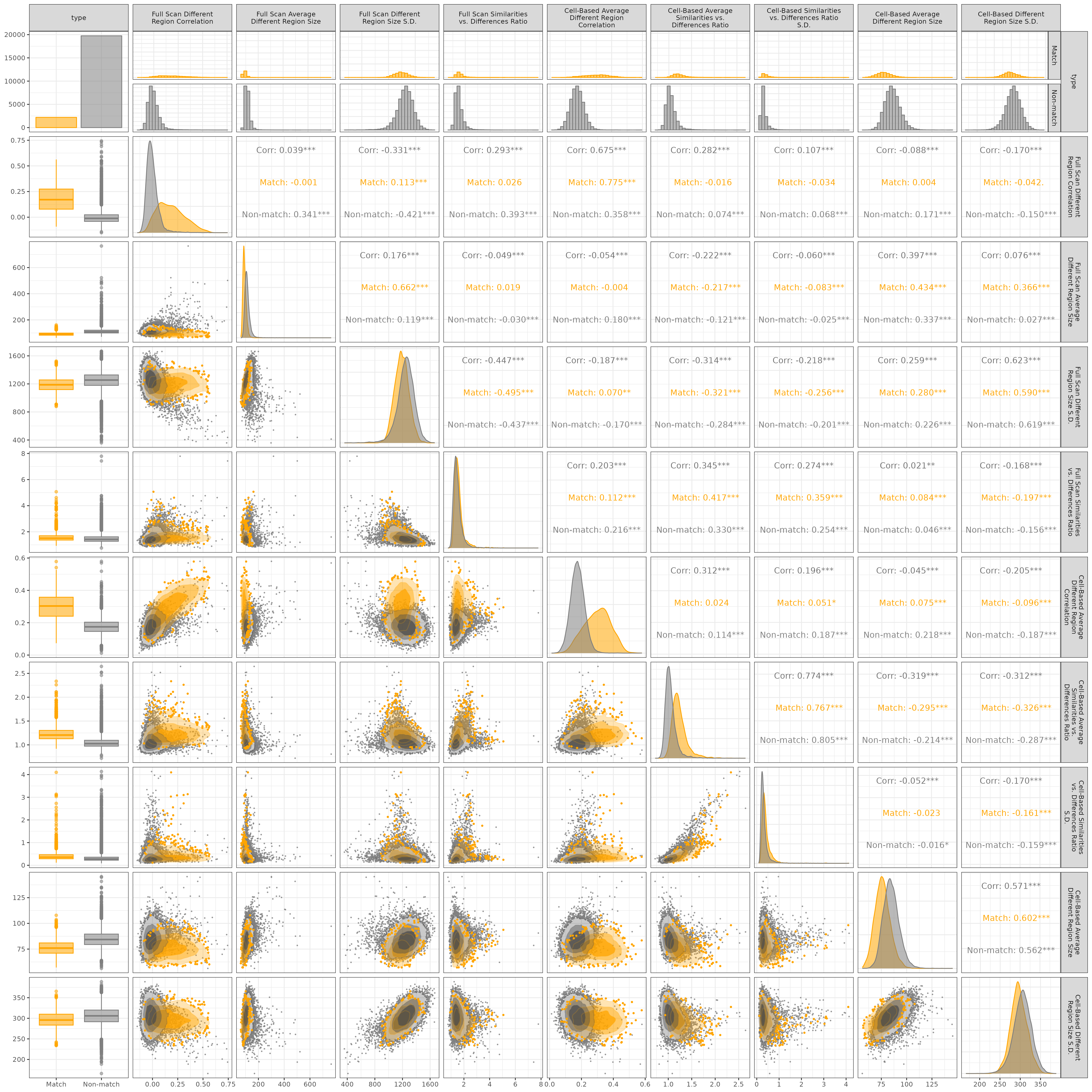
Figure 3.14: Pairs plot for visual diagnostic feature values computed for 2,189 matching and 19,756 non-matching pairwise comparisons.
Overall, there are only a handful of feature pairs that have strong linear relationships, and many of these exhibit different behavior between the matching and non-matching comparisons. This indicates that the discriminatory power of one feature isn’t fully accounted for by that of another feature and that each feature can more or less stand on its own merits to be included in a statistical model. In the next section, we explore results from fitting and testing binary classifiers using the visual diagnostic features.
3.4.2 Binary Classification Results
Using the 21,945 training comparisons, we train three binary classifier models: based on a decision tree (Breiman et al. 2017; Therneau and Atkinson 2022), random forest (Breiman 2001; Liaw and Wiener 2002), and logistic regression (R Core Team 2023). Note that do not intend to present a “final” model recommendation that should be used in forensic casework here - our present goal is merely to explore the discriminatory power of these nine visual diagnostic features. See Chapter 4 for a broader exploration of cartridge case similarity scoring algorithms.
Using the caret R package (Kuhn 2022), we perform 10-fold cross-validation, repeated three times, to train each model.
Ultimately, we choose the model that maximizes the area under the receiver operating characteristic (ROC) curve, abbreviated “AUC.”
We consider fitting each of the three classifier models to three subsets of the nine visual diagnostic features introduced in the last section: only the 4 full scan features, only the 5 cell-based features, and all 9 visual diagnostic features.
This helps us understand the relative discriminatory power of the full scan an cell-based features, as well as their utility when combined.
Finally, we also explore the use of up-sampling the matching comparisons and down-sampling the non-matching comparisons as a means of addressing the class imbalance in the training and testing data.
Note that this sub-sampling is performed within the re-sampling of the 10-fold cross-validation.
For comparison, we also fit each model without any sub-sampling.
In total, we train 27 models (3 classifiers \(\times\) 3 feature groups \(\times\) 3 sampling techniques) using the 10-fold, thrice-repeated cross-validation.
Figure 3.15 shows ROC curve and AUC results for the 27 classifiers. Comparing first across models (columns), we see that the random forest and logistic regression models have notably higher AUC values compared to the decision tree (CART) models. In fact, the random forest model achieves perfect training classification, as evidenced by the AUC values equal to 1, when either no sampling is performed or the matching comparisons are up-sampled. It makes sense that the random forest performs better than the CART model, since a random forest consists of an ensemble of CART models. It is surprising that the logistic regression classifier performs comparable to the random forest due to its relative simplicity. Considering sub-sampling procedures (rows), we see that the behavior of the AUC differs across the three models. For the CART model, performing either sub-sampling techniques resulted in higher AUC values compared to no sampling. The random forest and logistic regression models are comparatively much more consistent.
Finally, across feature groups (color) we see for the logistic regression and random forest models that the AUC is largest when all 9 visual diagnostic features are used. For the logistic regression model, training based on the 4 full scan features results in the lowest AUC values, followed by the 5 cell-based features, and finally all 9 features. Considering the feature distributions along the main diagonal of Figure 3.14, we note that features including the cell-based different region correlation and average similarities vs. differences ratio appear to yield greater separation between matching and non-matching comparisons than the full scan versions of these features. For generalized linear models like the logistic regression classifier, it makes sense that the greater separation for the cell-based features would to better classification results over the full scan features. However, the fact that the random forest achieves an AUC of 1 based on both the full scan and cell-based features indicates that there is a non-linear decision boundary in both feature spaces that perfectly separates matches from non-matches. It isn’t a surprise that training the random forest on the combined features also results in an AUC of 1.
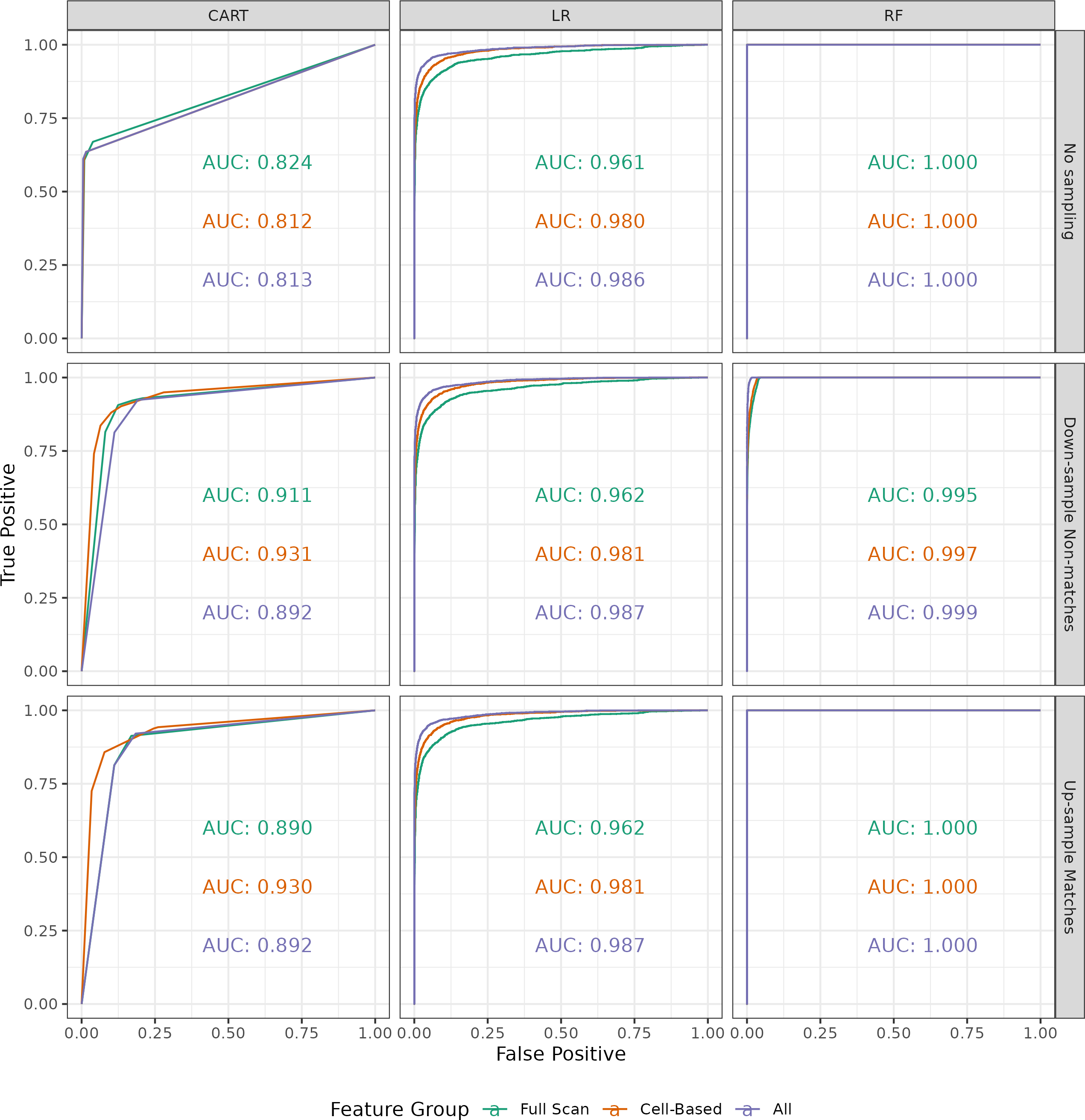
Figure 3.15: ROC curves for three binary classifier models (columns) trained using three sampling schemes (rows) on three subsets of the 9 visual diagnostic features (color). Overall, the random forest models have the highest AUC, specifically achieving perfect training classification when either no sampling is performed or the matching comparisons are up-sampled. The logistic regression models perform second best and is relatively invariant to sub-sampling scheme. The decision tree (CART) models have considerably lower AUC values overall and are sensitive to sub-sampling scheme. For the random forest and logistic regression models, using all 9 visual diagnostic features leads to higher AUCs compared to the smaller subsets, except for when the AUCs are all 1.
Consider the distributions of training match probabilities shown in Figure 3.16, distinguished by firearm ID pair. These match probabilities are computed using the random forest model trained on all 9 visual diagnostic features without any sub-sampling. We distinguish the 10 training firearm IDs by rows/columns, meaning the main diagonal plots show match probabilities for the truly matching comparisons while the off-diagonal plots show the same for non-matching comparisons. The horizontal axis for all plots represents the estimated match probability for all pairwise comparisons between scans from “Firearm 1” (columns) and scans from “Firearm 2” (rows). Note that we transform the horizontal axis according the density of a Beta(4,4) distribution under the canonical shape Beta distribution parameterization. Considering that we draw horizontal axis breaks (gray vertical lines) at \(\{0, 0.25, .5, 0.75, 1\}\), this transformation causes a “stretching” of values near 0 and 1 and “contracting” of values near 0.5. We perform this transformation to provide a clearer visual of the match probabilities, which tend to “bunch up” near the extremes of the interval. The vertical axis represents the density of the match probabilities for the density plots in the main diagonal and upper-triangle. Because the pairwise match probability is invariant to which firearm is labeled “1” or “2,” the box plots in the lower-triangle depict the same data in the upper-triangle. We combine the box plot and densities for the matching comparisons along the main diagonal.
Considering the matching to non-matching distributions, we see that the match probabilities tend to be more variable than the non-match probabilities. For example, matching Firearm Z comparisons have associated match probabilities ranging from 0.6 to 1.0 with a median probability value of 0.8. Comparatively, the non-match comparisons are more strongly right-skewed - the classifier is more “sure” when a pair doesn’t match. About 15% (338 of 2,199) of all matching comparisons and 49% (9693 of 19,756) of all non-matching comparisons have an assigned match probability of 1.0 and 0.0, respectively. In the case of the random forest classifier, this simply means that none of the constituent, ensembled decision tree classifiers “voted” for the incorrect class for these comparisons, but this further underscores the match vs. non-match imbalance. We considered the feature distributions of these specific comparisons and noted that they exhibited excellent separation in a few, key features - namely, the full scan and cell-based difference correlations - that the random forest also considered highly “important” as measured by the mean Gini Index decrease (Liaw and Wiener 2002). In contrast, matching comparisons from Firearm Z exhibit poorer separation in these important features compared to non-match comparisons, which explains the lower match probabilities in Figure 3.16.
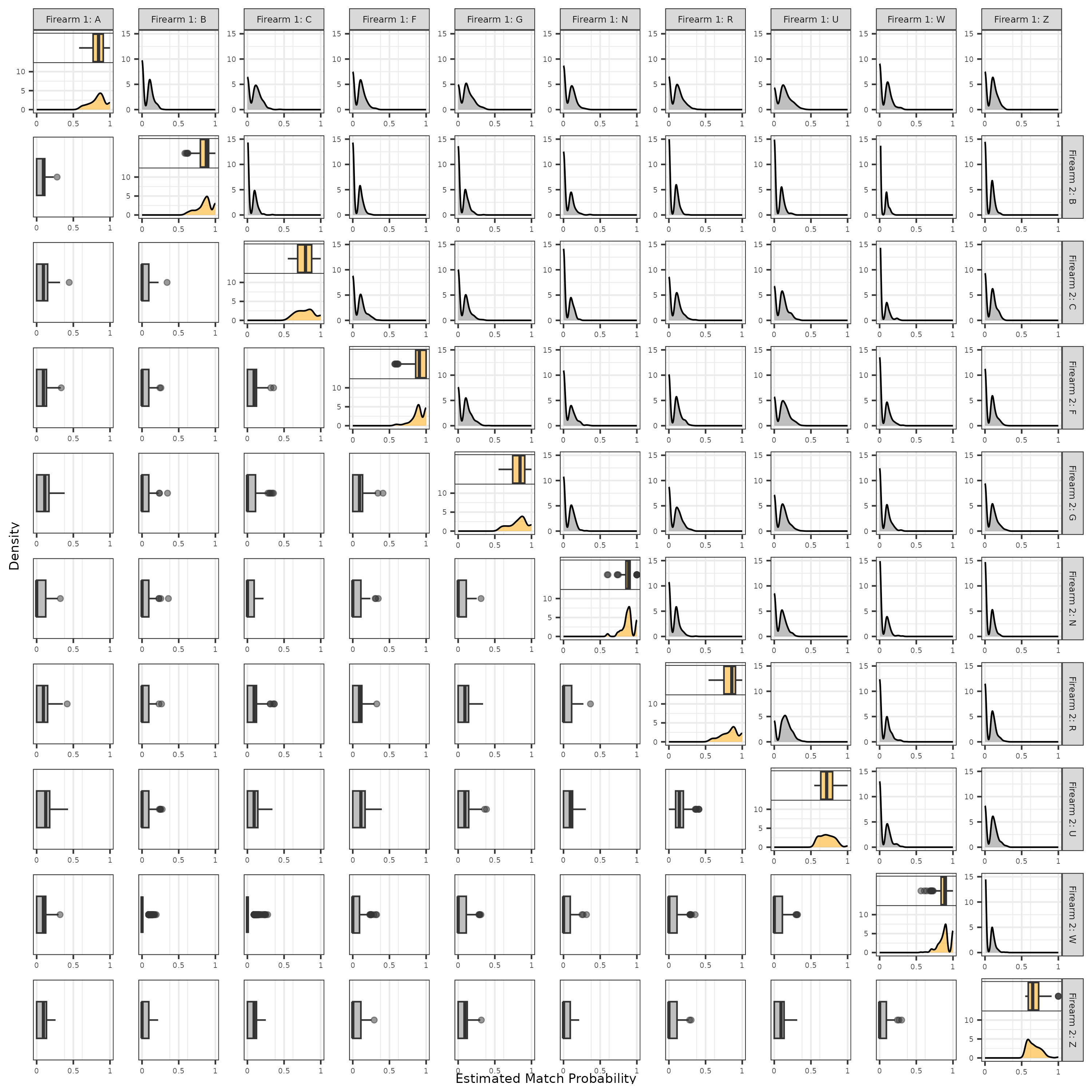
Figure 3.16: Distribution of match probabilities estimated using a random forest classifier. We distinguish these probabilities by firearm ID pair, meaning each plot represents the pairwise comparisons in which one cartridge case originated from the “column” firearm and the other from the “row” firearm. Matching comparisons are represented along the main diagonal plots while non-match comparisons are shown in the off-diagonal.
3.5 Discussion
3.5.1 Case Studies
In this section, we explore specific examples of cartridge case comparisons to understand the relationship between qualitative observations we can make using the visual diagnostic tools and the quantitative measures of similarity we obtain from a binary classifier. The phenomenon of classifier models not being as adept at identifying matching comparisons has been observed in many other cartridge evidence scoring methods (Song 2013; Chen et al. 2017) and Chapter 4. There are a variety of factors that may lead to this discrepancy, but one of the most important factors that we’ve identified is whether extraneous, non-breech face markings are correctly identified and removed during pre-processing. We have consistently noted that extreme values in a scan tend to heavily impact the registration procedure. For example, when applying the cell-based comparison procedure of cell-based comparison, large markings in the target scan seem to “attract” source cells, even if those cells do not contain similar markings when visually compared. Diagnostic tools like the X3P and Comparison plots are useful for understanding why a cell registers in these areas.
We return to the pair of matching cartridge cases shown in Figure 3.5. Recall that we computed the cross-correlation function (CCF) between these scans before and after extraneous, non-breech face observations were removed from the scans. Removing the non-breech face impressions made it easier to visually identify similar impressions between the two scans and increased the CCF value, implying higher similarity. We now consider the similarity score for between these two scans estimated using the random forest binary classifier. The left side of Figure 3.17 shows the cell-wise registrations for this comparison using K002eG2 as reference and K227iG3 as target. Similar to Figure 3.5, the top and bottom show results from two cases: before and after removing the non-breech face observations from the two scans. Estimating a similarity between these two scans using the “no sampling,” “all features” random forest classifier results in similarity scores of 0.66 and 1.00, respectively, for these two cases.
The source cells align in a more grid-like pattern in “K227iG3 + Additional Pre-processing” than in “K227iG3 Original”, where the extreme values along the inner rim seem to “pull” cells towards the center. Cells like 1, 1 or 1, 4 do not register in a grid-like pattern in either case, although the registration in the “Additional Pre-processing” case is easier to justify as being due to the removal of observations in that region of K227iG3. We would rather a registration fail due to a lack of shared information between the two scans than due to spurious similarities between extreme values. As a specific example, we we depict the comparison plot for cell 3, 4 with its aligned mate in the target scan on the right side of Figure 3.17. In the “original” case, we see that cell aligns to the non-breech face values along the inner rim of K227iG3. The filtered element-wise average between these cells actually does uncover some similarities, such as the faint orange values on the upper-right side of the two scans, yet these are insignificant compared to the large dissimilar regions in the center of the cells. In contrast, the similarities are much more obvious in the “Additional Pre-processing” case based on the deeper purple/orange shades in the filtered element-wise average plot. Further, careful study of the filtered differences between these cells shows that there are similar trends between the different regions of these scans, which upholds the use of the “differences correlation” feature.
This example demonstrates how the visual diagnostic tools both corroborate and inform the results from a trained classifier model. Both the visual diagnostics and algorithm-based similarity score indicate that the original versions of the scans are not particularly similar. However, only the visual diagnostics indicate that the dissimilarity is due to the presence of observations that “distract” the algorithm from comparing the actual breech face markings. Upon removing these observations, both the visual diagnostics and similarity score reflect the similarity between the breech face impressions.
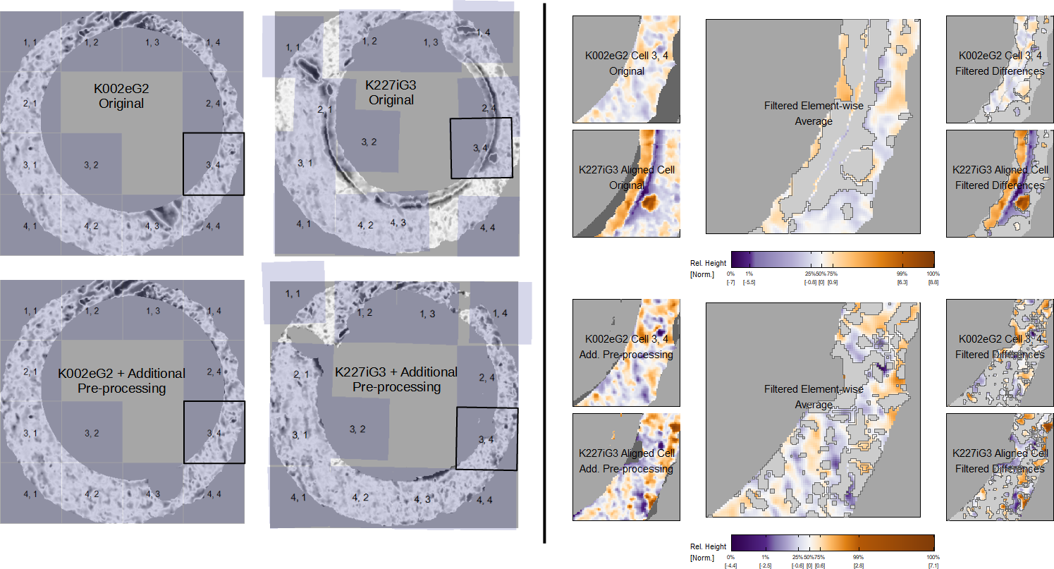
Figure 3.17: Aligned cells from the matching comparison shown in 3.5. In the top row, non-breech face values are left in the scan, which leads to poor alignment of cells and an overall low similarity score (0.66). In the bottom row, we remove the non-breech values, which leads to improved alignment and a higher similarity score (1.00). In both cases, we show the comparison plot for cell 3, 4 and note that similar markings are more easily identified once the extraneous observations are removed. This illustrates how removing “distracting” values from the cartridge case scans during pre-processing can improve downstream similarity results.
Next, we consider cartridge cases pairs that exhibited behavior in their similarity scores. Specifically, we consider the matching and non-matching comparisons with the smallest and largest associated similarity score, respectively, as computed by the “no sampling,” “all features” random forest model. These examples help us understand conditions under which the algorithm doesn’t behave as desired. The first row of Figure 3.18 shows matching K011sR1 and K046uR2 that have an estimated similarity score of 0.59. The second row of Figure 3.18 shows non-matching K013pC1 and K027gA3 that have an estimated similarity score of 0.38. Compared to the matching comparison between K002eG2 and K227iG3, it is harder to identify similar, distinctive impressions for these two pairs. For example, the surfaces of both K011sR1 and K046uR2 appear more mottled with small-scale markings than imprinted with large striations like those visible in K002eG2 and K227iG3. There are some striated markings visible in the north-east corner of scan K027gA3, but the same region in K013pC1 has only a thin strip of observations. As such, there isn’t enough shared information in this region to say confidently that the impressions are similar or different. The remaining surface of these two scans are similar to K011sR1 and K046uR2 in that there aren’t particularly distinctive markings. A case could be made to apply additional pre-processing to remove the arc of orange and purple values along the south to south-west outer edge in K046uR2, but we don’t expect the results to change drastically.
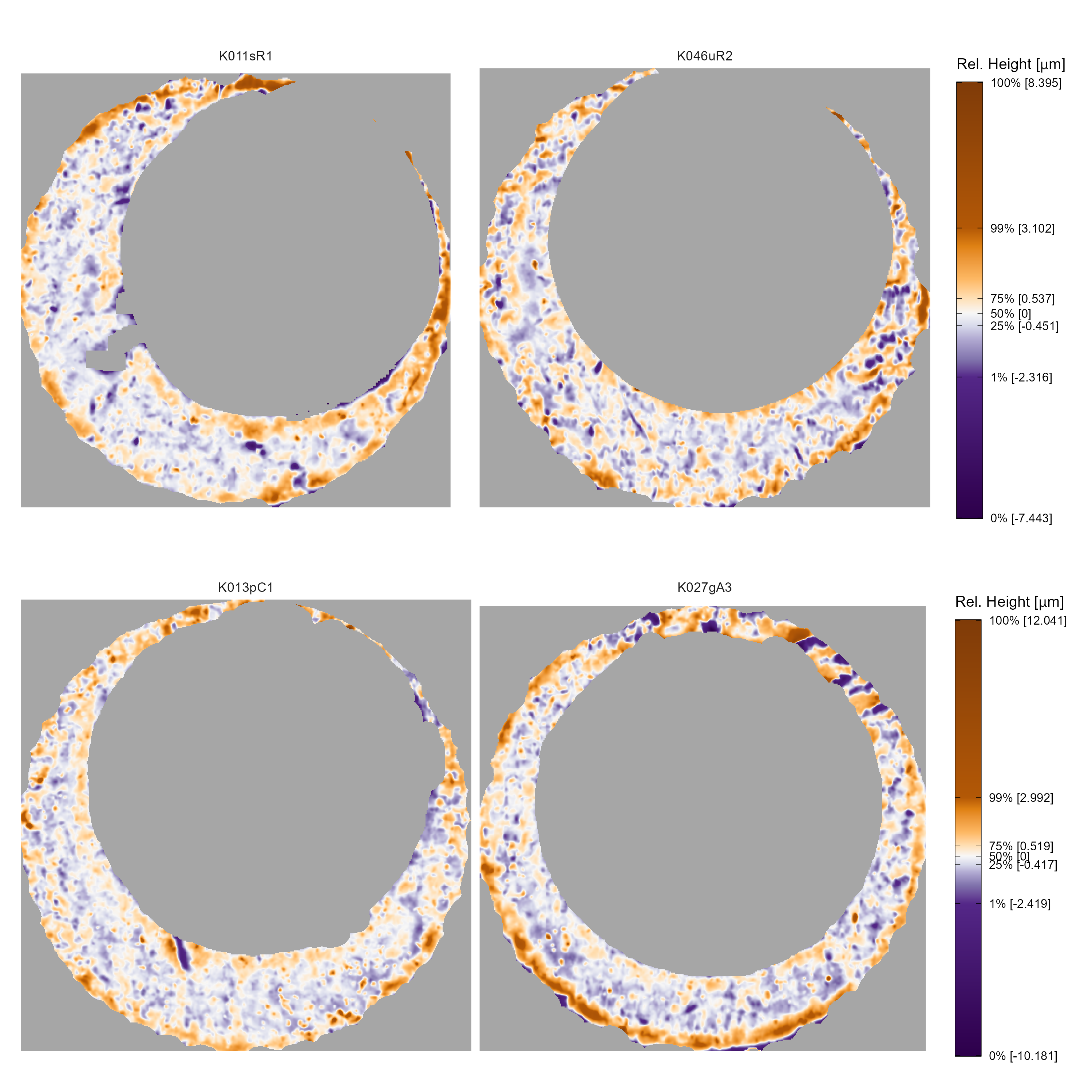
Figure 3.18: In the first row, we show the pair of matching scans with a low similarity score of 0.59. In the second row, we show a pair of non-match scans with a relatively high similarity score of 0.38. In both cases, the associated similarity scores seem attributable not to definite similarities or dissimilarities, but instead to a lack of distinctive markings.
As further support for the middling similarity scores for these two pairs, consider Figure 3.19 that shows numerical feature and score values for the 21,945 comparisons considered in the last section. On the left, we visualize the densities for the 9 visual diagnostic feature values - these are the same as the densities shown in Figure 3.14. On the right, we visualize the similarity score densities - this is a combination of the densities shown in Figure 3.16. On top of each density plot, we visualize the value associated with the two pairs considered in Figure 3.18 as an orange (match) and black (non-match) line. This visual allows us to compare the feature values of these specific match and non-match pairs to each other and to the rest of the 21,943 pairwise comparisons.
We see that many feature values associated with these pairs fall between or around the modes of the matching and non-matching densities, which suggests that none of the features clearly exhibit the behavior of a matching or non-matching comparison. The two pairs are “unexceptional” based on these features, which explains why the are assigned similarity scores close to the middle of the interval. Interestingly, if we compare the two lines to each other across the various feature densities, we see that the non-match comparison between K013pC1 and K027gA3 has feature values more similar to a match comparison than the actually matching comparison between K011sR1 and K046uR2. For example, we expect the cell-based average different region correlation (top-left) to be large if two cartridge cases match. In this instance, however, the non-match comparison has a larger associated correlation value, 0.26, than that of the match comparison, 0.22. Only for the cell-based average difference region size (top-center) and the standard deviation of the full scan difference region sizes (bottom-center) does the match comparison “look” more like a match comparison. Despite this, the similarity score associated with the match comparisons is still larger than that of the non-match comparison. This suggests the existence of higher-order interactions between these 9 features that aren’t obvious from a one-dimensional density plot, but that can be “learned” by the random forest classifier model. For example, the lower-diagonal of the pairs plot in Figure 3.14 shows the pairwise relationship of some features differs for matching vs. non-matching comparisons.
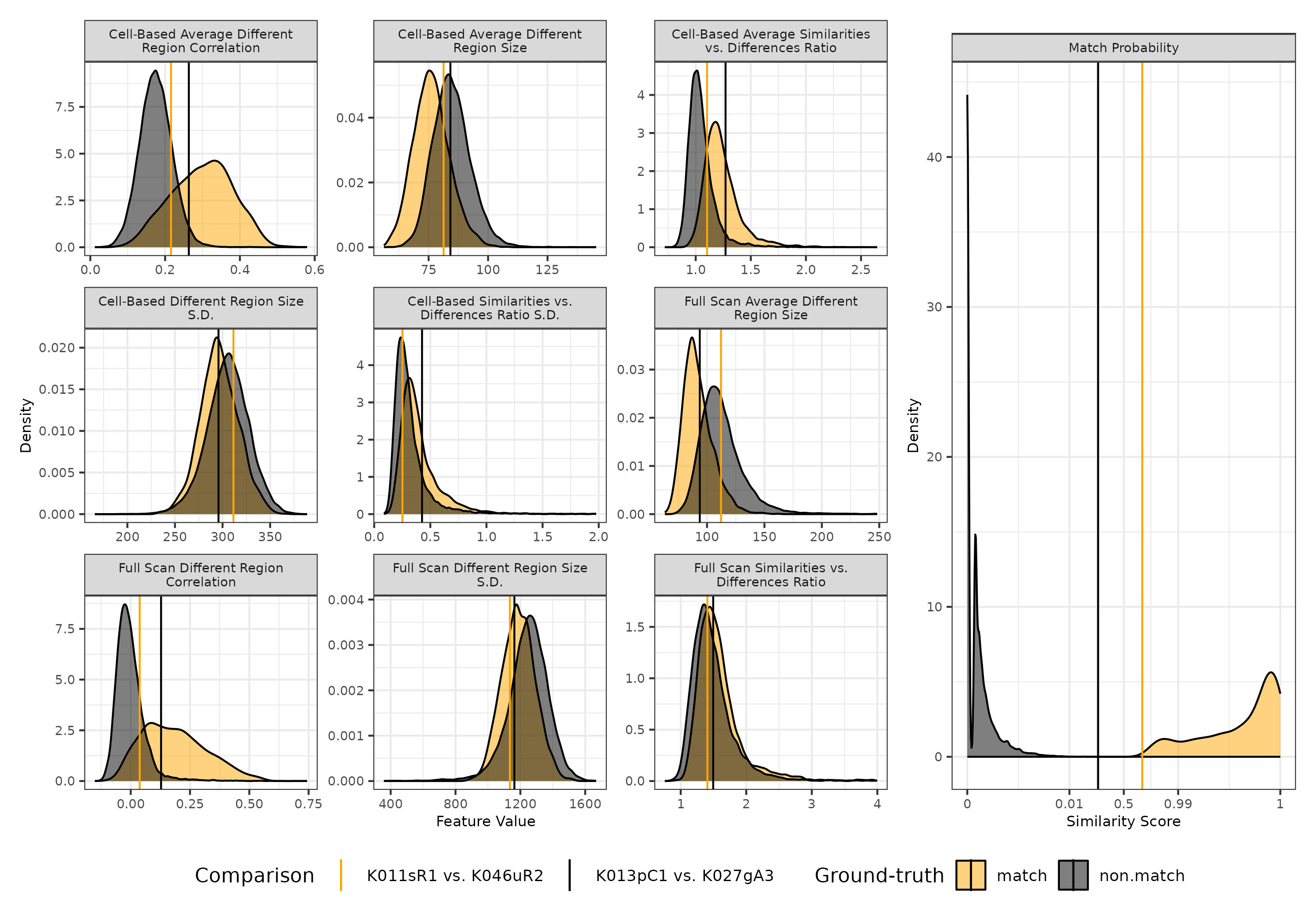
Figure 3.19: Density plots of 9 visual diagnostic features (left) and estimated similarity score (right) for 21,945 pairwise comparisons, distinguished by match and non-match comparisons. On top of each plot we visualize the values associated with the two cartridge case pairs shown in Figure 3.18. We see that the feature values for these two pairs fall close to the intersection of the match and non-match densities, which suggests the cartridge cases are fairly unexceptional. This explains the middling similarity scores observed in the right plot.
Finally, we consider the non-match cartridge case pair K013sA3 and K015iZ2, which has the largest value for the full scan average different region size feature of 765 pixels. We see that the estimated registration of these two scans leads to very little overlap between the non-missing values. The observations that do overlap appear to do so because of striated markings that appear on the two surfaces, although studying these markings reveal that they look quite dissimilar. Consequently, the filtering operation leads to only a few neighborhoods of filtered values, although they are each relatively large. This explains the large filtered neighborhood feature value associated with this comparison. These scan illustrate how the phenomenon of an “obvious” non-match, sometimes observed in firearm and toolmark casework, might appear when applying a registration algorithm.
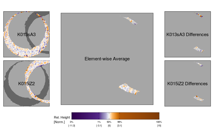
Figure 3.20: Comparison plot for two non-matching scans K013sA3 and K015iZ2. The estimated registration of these two scans leads to very little overlap betwen the non-missing values of the two scans. This demonstrates how an “obvious” non-match cartridge case pair can appear when applying the image registration algorithm.
3.5.2 Software
We developed an interactive web application called cartridgeInvestigatR to give non-programmers access to the visual diagnostic tools. The application is accessible at https://csafe.shinyapps.io/cartridgeInvestigatR/. For a guide on using the application, visit https://github.com/jzemmels/cartridgeInvestigatR.
We also created a package called impressions to implement the visual diagnostics in the R programming language.
You can currently install impressions from GitHub at https://github.com/jzemmels/impressions, although we plan to submit the package to CRAN soon.
See https://jzemmels.github.io/impressions/ for more information.
3.6 Conclusion
Algorithms rarely have built-in mechanisms to determine when they work as expected, so diagnostic tools aid the user in understanding when human intervention into the algorithmic pipeline is needed. In this paper, we introduced a suite of diagnostic tools to explore each step of a cartridge case comparison algorithms. These visual diagnostics can be used both as a quick reference to determine whether changes to earlier stages of the pipeline are warranted and as a tool to carefully study the behavior of the algorithm.
We discussed how non-breech face markings that are kept in the scan after pre-processing may be distracting to the full scan or cell-based registration procedures. The X3P plot is a particularly useful tool to check for necessary pre-processing because it emphasizes extreme surface values. After registering full scans or cells, the Comparison plot is useful to analyze specific regions of the scans for similarities and differences. To better understand the output of a similarity scoring algorithm, the visual diagnostic statistics provide a quantitative complement to the qualitative observations drawn from the other diagnostic tools. We demonstrated that these features are effective at distinguishing between matches and non-matches under a variety of conditions, which lends further credibility to their use as diagnostic tools and indicates that they could be useful in a statistical classification algorithm. We discuss this further in Chapter 4.
We anticipate that these diagnostic tools will be used iteratively to check that each of the three major stages of a comparison algorithm - pre-processing, comparing, and scoring - hasn’t obviously gone awry. For example, the user might visualize a pre-processed cartridge case using the X3P plot only to realize that further pre-processing is needed to remove extraneous information. After applying additional pre-processing, the user can return to the X3P plot to ensure that the extraneous information was removed. We recognize that ground-truth is unknown in actual casework, so it may be challenging to differentiate between extraneous markings and genuine breech face impressions. As such, we will continue to work with forensic examiners to better understand the nature of the evidence they commonly see and develop the diagnostic tools and cartridgeInvestigatR to better suite their needs.