Appendix

4.7 Registration Procedure Details

In our application, a registration is composed of a discrete translation by \((m,n) \in \mathbb{Z}^2\) and rotation by \(\theta \in [-180^\circ,180^\circ]\). Under this transformation, the index \(i,j\) maps to a new index \(i^*,j^*\) by:

\[\begin{align*} \begin{pmatrix} j^* \\ i^* \end{pmatrix} = \begin{pmatrix} n \\ m \end{pmatrix} + \begin{pmatrix} \cos(\theta) & -\sin(\theta) \\ \sin(\theta) & \cos(\theta) \end{pmatrix} \begin{pmatrix} j \\ i \end{pmatrix}. \end{align*}\]

The value \(b_{ij}\) now occupies the index \(i^*, j^*\). In practice, we use nearest-neighbor interpolation meaning \(i^*\) and \(j^*\) are rounded to the nearest integer.

To determine the optimal registration, we calculate the cross-correlation function (CCF) between \(A\) and \(B\), which measures the similarity between \(A\) and \(B\) for every possible translation of \(B\). Denoted \((A \star B)\), the CCF between \(A\) and \(B\) is a 2D array of dimension \(2k - 1 \times 2k - 1\) with the \(m,n\)-th element given by:

\[ (a \star b)_{mn} = \sum_{i=1}^k \sum_{j=1}^k a_{mn} \cdot b_{i + m, j + n} \]

where \(1 \leq m,n \leq 2k - 1\). The value \((a \star b)_{mn}\) quantifies the similarity between \(A\) and \(B\) after \(B\) is translated \(m\) elements horizontally and \(n\) elements vertically. The CCF is often normalized between -1 and 1 for interpretability.

The above definition of the CCF is computationally taxing, particularly for large matrices. The Cross-Correlation Theorem provides an equivalent expression for the CCF:

\[ (A \star B) = \mathcal{F}^{-1}\left(\overline{\mathcal{F}(A)} \odot \mathcal{F}(B)\right) \]

where \(\mathcal{F}\) and \(\mathcal{F}^{-1}\) are the discrete Fourier and inverse discrete Fourier transforms, respectively, \(\overline{\mathcal{F}(A)}\) is the complex conjugate, and \(\odot\) is an element-wise (Hadamard) product (Brigham 1988). We trade the moving sum computation from the previous CCF expression for two forward Fourier transforms, an element-wise product, and an inverse Fourier transform. The Fast Fourier Transform (FFT) algorithm reduces the computational load considerably [cite Tukey].

We estimate the registration by calculating the maximum CCF value across a range of rotations of matrix \(B\). Let \(B_\theta\) denote \(B\) rotated by an angle \(\theta \in [-180^\circ,180^\circ]\) and \(b_{\theta_{mn}}\) the \(m,n\)-th element of \(B_\theta\). Then the estimated registration \((m^*,n^*,\theta^*)\) is:

\[ (m^*,n^*,\theta^*) = \arg \max_{m,n,\theta} (a \star b_\theta)_{mn}. \]

In practice we consider a discrete grid of rotations \(\pmb{\Theta} \subset [-180^\circ,180^\circ]\). The registration procedure is outlined in Image Registration Algorithm. We refer to the matrix that is rotated as the “target.” The result is the estimated registration of the target matrix to the “source” matrix.

The Fast Fourier Transform algorithm used in Image Registration Algorithm does not permit missing values in \(A\) or \(B\). It is common for cartridge case scans to contain many missing values - the gray regions in Figure 4.3 represent structural values in the scan. Thus, when calculating the CCF we impute these missing values with the average non-missing value in the scan. To measure the similarity between \(A\) and \(B\) while accounting for missingness, we calculate the correlation between the non-missing intersection of the aligned scans.

4.7.1 Cell-Based Registration Details

Following the full-scan registration, we next perform a cell-based registration procedure. Song (2013) points out that breech face impressions rarely appear uniformly on a cartridge case surface. Rather, distinguishing markings appear in specific, usually small, regions of a scan (the author refers to these as valid correlation regions). Calculating a correlation between two whole scans does not necessarily capture the similarity between these regions. Song (2013) proposes partitioning a scan into a rectangular grid of “cells” to isolate the valid correlation regions. Figure 4.4 shows an example of two non-match cartridge cases where the source matrix (left) is partitioned into an \(8 \times 8\) grid of cells.

The cell-based comparison procedure begins with selecting one of the matrices, say \(A\), as the “source” matrix to be partitioned into a grid of cells. Each of these source cells will be compared to the “target” matrix, in this case \(B^*\). Because \(A\) and \(B^*\) are already partially aligned based on the course rotation grid \(\pmb{\Theta}\), we compare each source cell to \(B^*\) using a new rotation grid of \(\pmb{\Theta}'_A = \{\theta^*_A - 2^\circ, \theta^*_A - 1^\circ,\theta^*_A,\theta^*_A + 1^\circ,\theta^*_A + 2^\circ\}\).

If two cartridge cases are truly matching, then we assume that multiple cells will “agree” on a particular translation value at the true rotation. This agreement phenomenon is illustrated in Figure 4.13 where each point represents the translation that maximizes the CCF for a particular cell and rotation. The points appear randomly distributed for most of the rotation values except around \(\theta = 3\) where a tight cluster of points forms around translation \([m,n] \approx [17,-16]\). This is evidence to suggest that a true registration exists for these two cartridge cases, implying that they match. The task is to determine when cells reach a registration consensus.

Figure 4.13: A scatterplot where points represent the cell-wise estimated translations faceted by rotation for a matching pair of cartridge cases. As evidenced by the tight cluster in the middle facet, it appears that multiple cells agree on a translation of \([m, n] \approx [17,-16]\) after rotating by \(3^\circ\). Points are jittered for visibility.

4.7.2 Registration-Based Feature Distributions

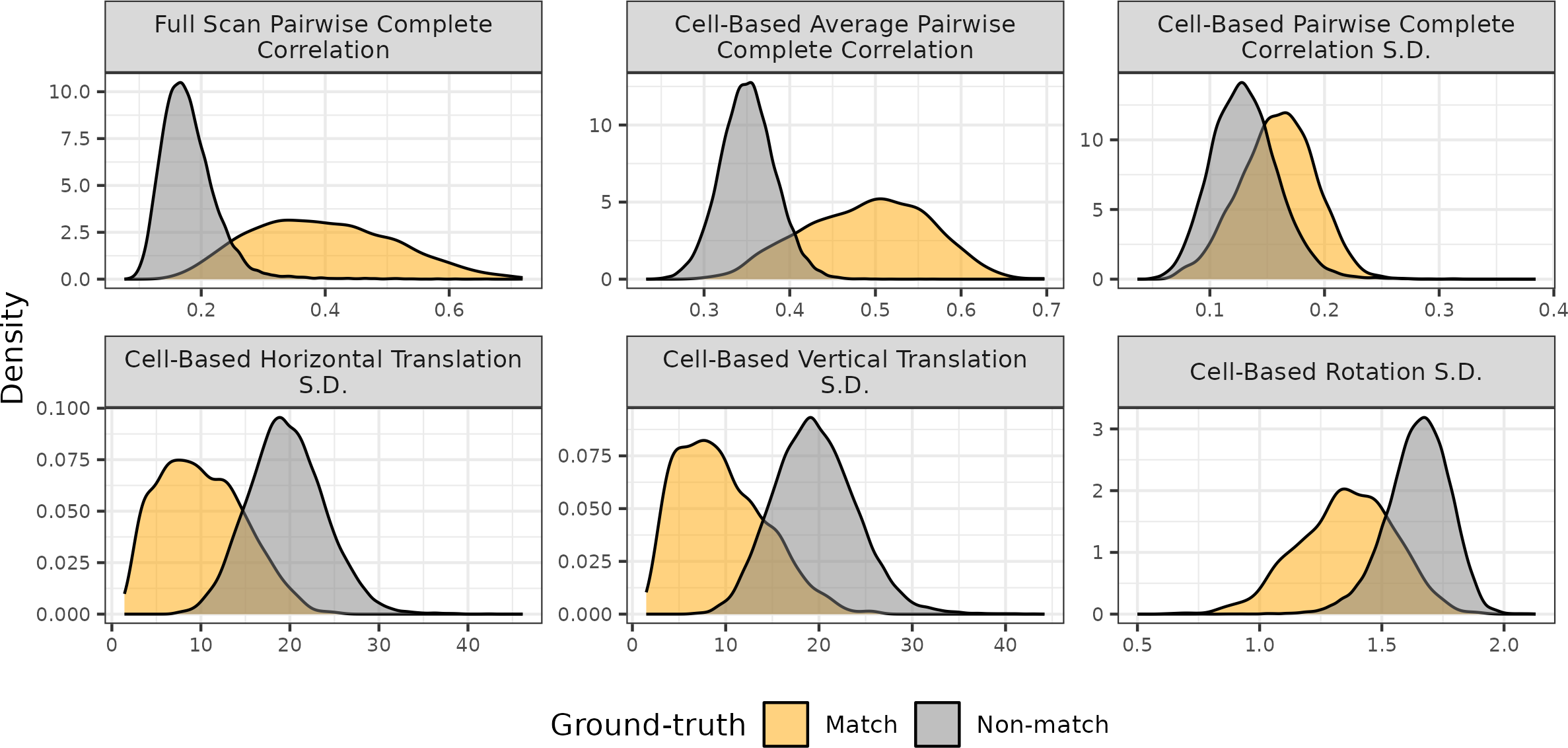
Figure 4.14 shows density plots of the registration-based features for 21,945 cartridge case pairs. The first two rows show densities for the sample mean and standard deviation of the cell-based registrations, respectively. The third row shows densities for the pairwise-complete correlation features.

Figure 4.14: Density plots of the Registration-Based features for 21,945 cartridge case pairs. The standard deviation of the cell-based registrations distinguish between match and non-match pairs better than the mean values.

4.7.3 Density-Based Feature Distributions

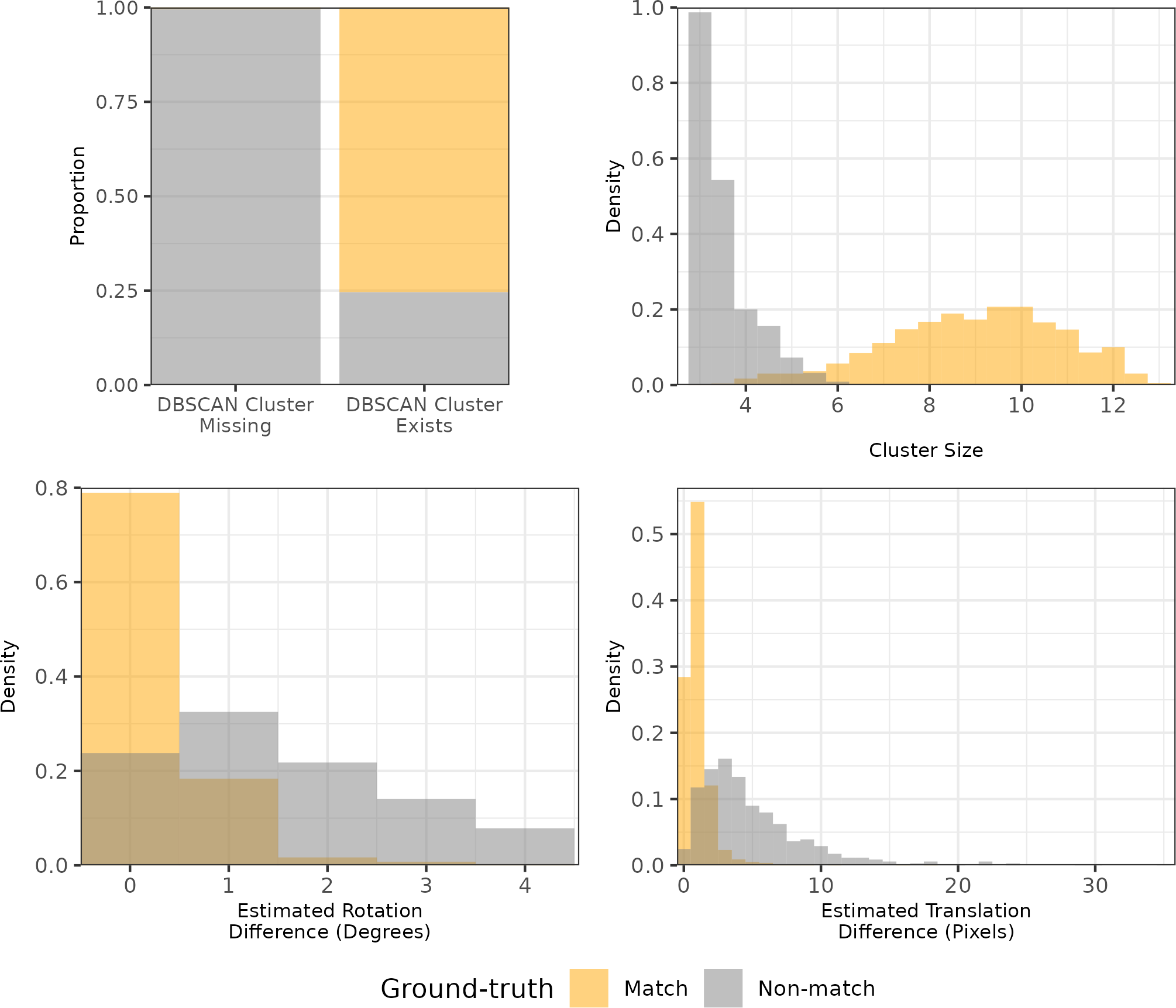
Figure 4.15 shows the distributions of the density-based features \(C\), \(\Delta_\theta\), and \(\Delta_{\text{trans}}\). The stacked bar chart in the top-left shows the proportion of comparisons where no DBSCAN cluster is identified by outcome (match or non-match). We see that the vast majority of comparisons for which no DBSCAN cluster is identified are non-match comparisons. indicating that \(C_0\) is a good indicator of ground-truth. In fact, there is only one non-match comparison that resulted in a DBSCAN cluster. It’s difficult to see in the plots, but the \(C\) value for this non-match pair is 5 and the \(\Delta_{\text{trans}}\) value is 23.9. As expected, \(C\) tends to be relatively large for matching comparisons while \(\Delta_{\theta}\) and \(\Delta_{\text{trans}}\) tends to be small.

Figure 4.15: Distributions of the density-based features for 21,945 cartridge case pairs. The Cluster Size and Estimated Translation Difference features may be missing () if no DBSCAN cluster is identified, which commonly occurs for non-matching cartridge case pairs as evidenced by the stacked bar chart in the top left. This explains the near absence of non-matching comparisons from Cluster Size and Estimated Translation Difference plots. Whether a cluster is identified for a particular comparison strongly predicts whether it is a match or a non-match, which justifies the inclusion of the cluster indicator feature \(C_0\).

4.7.4 Visual Diagnostic Feature Distributions

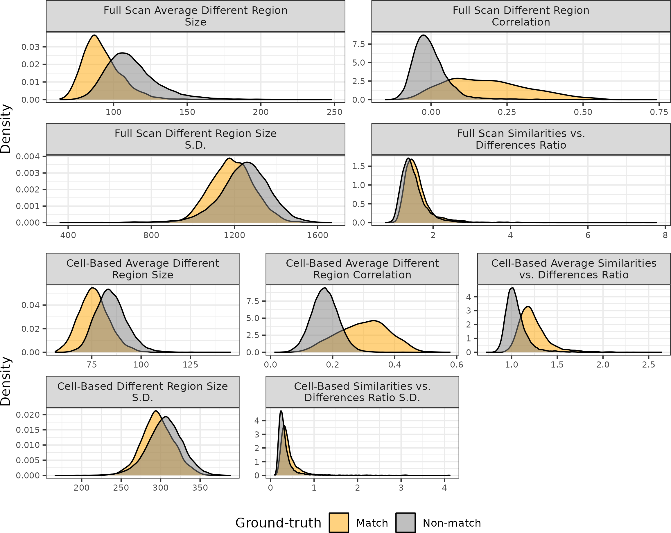
Figure 4.16 shows the distribution of the six visual diagnostic-based features. As expected, matching comparisons at the full-scan and cell-based levels tend to have smaller neighborhood sizes and higher correlation values on average.

Figure 4.16: Distributions of the visual diagnostic-based features for 21,945 cartridge case pairs. Matching comparisons tend to have smaller neighborhood sizes on average and higher correlation values than non-matches indicating their utility in a classifier.

4.8 Model-Specific Results

Table 4.6 summarizes the accuracy, true positive, and true negative rates based on the training data for the five binary classifier models.

Table 4.6: Accuracy, True Positive, and True Negative rates based on the training data for the 13 binary classifier models. This table shows a numeric summary of the results shown in the Results section. We bold the largest values in each column for emphasis.

Feature Set	Model	Accuracy	True Neg.	True Pos.
\(C_0\)	Baseline	90.47	90.43	90.77
\(C_0\)+Registration	RF	97.16	97.15	97.18
\(C_0\)+Registration	LR	97.23	97.23	97.23
All~ACES	RF	98.14	98.14	98.14
All~ACES	LR

Table 4.7 summarizes the accuracy, true positive, and true negative rates based on the test data for the 13 binary classifier models.

The true positive rates for the test data are noticeably lower to those for the training data summarized in Table 4.6, although the true negative rates are similar.

Table 4.7: Accuracy, True Positive, and True Negative rates based on the test data for the 13 binary classifier models. This table shows a numeric summary of the results shown in the Results section. We bold the largest values in each column for emphasis.

Feature Set	Model	Accuracy	True Neg.	True Pos.
\(C_0\)	Baseline	89.44	89.64	86.82
\(C_0\)+Registration	RF	96.91	97.11	94.22
\(C_0\)+Registration	LR	96.98	97.21	93.87
All~ACES	RF	97.66		94.74
All~ACES	LR		97.81

References

Brigham, E. Oran. 1988. The Fast Fourier Transform and Its Applications. USA: Prentice-Hall, Inc.

Song, John. 2013. “Proposed ‘NIST Ballistics Identification System (NBIS)’ Based on 3d Topography Measurements on Correlation Cells.” American Firearm and Tool Mark Examiners Journal 45 (2): 11. https://tsapps.nist.gov/publication/get_pdf.cfm?pub_id=910868.