scored

As an example, consider two cartridge cases fired from the same Ruger SR9 semiautomatic 9-mm handgun. Learn more about the collection of these cartridge cases here. The cartridge cases are uniquely identified as “K013sA1” and “K013sA2.” We assume that the markings on these cartridge cases left by the handgun during the firing process are similar.

library(scored)

library(cmcR)
library(impressions)
library(tidyverse)

data("K013sA1","K013sA2")

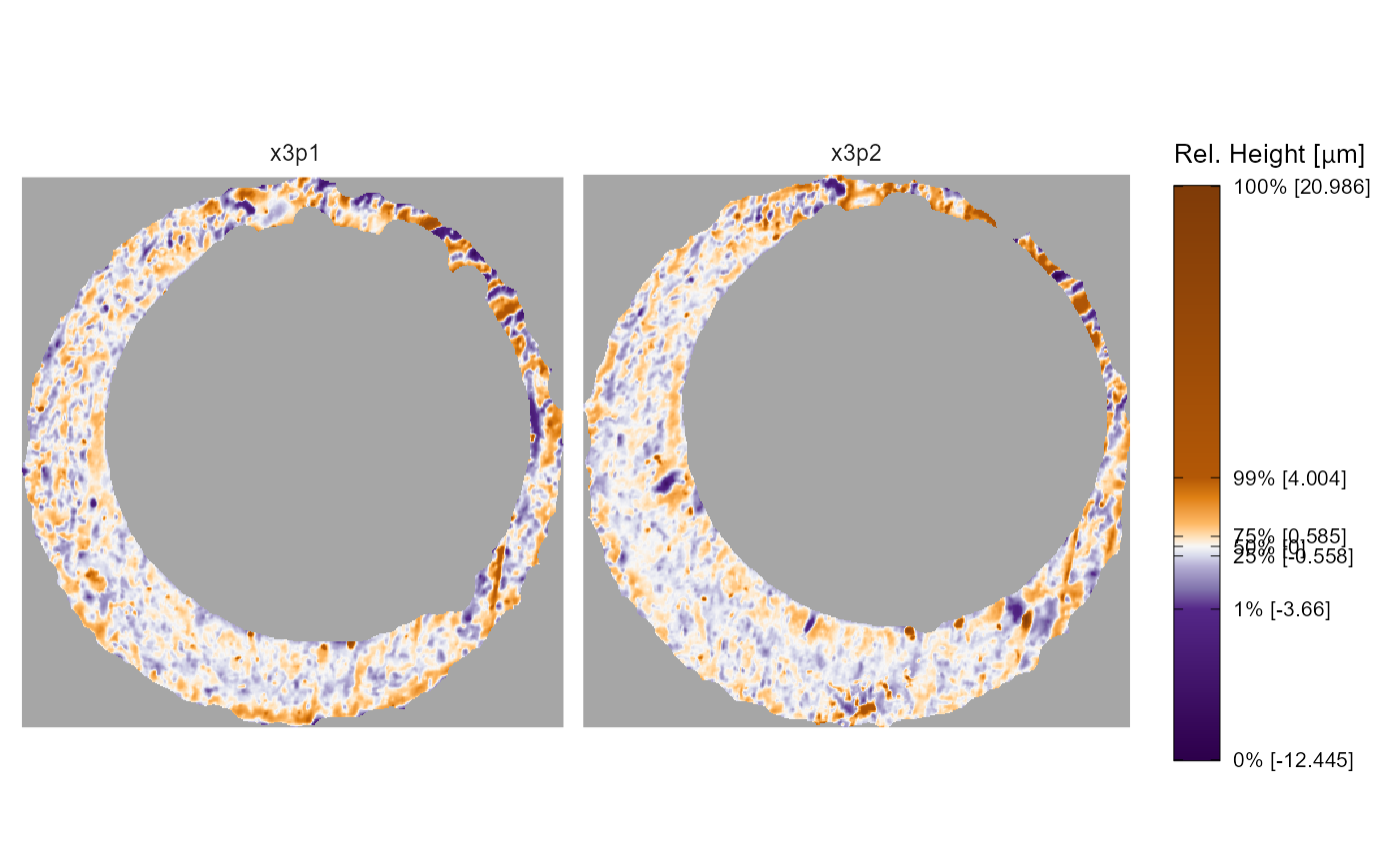
Below is a visual of the two cartridge case scans. Note that these scans have already undergone some preprocessing to emphasize the breech face impression markings. The similarity between these cartridge cases is not immediately apparent. We can calculate similarity features between these two scans using functions available in the scored package.

x3pPlot(K013sA1,K013sA2)

First, we compare the two scans using the cell-based comparison procedure implemented in the cmcR R package. Briefly, this cell-based comparison involves dividing one scan into a grid of “cells” and identifying the rotation/translation at which each cell aligns best in the other scan. This comparison is repeated in both directions: K013sA1 is divided into cells that are compared to K013sA2, and then K013sA2 is divided into cells that are compared to K013sA1. The resulting comparisonData data frame contains features related to the alignment of each cell in the other scan. By itself, the features in comparisonData are quite noisy – it’s difficult to measure the similarity between K013sA1 and K013sA2. The scored package contains functions that accept the comparisonData features as input and return more informative similarity features.

comparisonData <- comparison_cellBased(reference = K013sA1,target = K013sA2,
                                       thetas = seq(-30,30,by = 3),
                                       direction = "both",
                                       returnX3Ps = FALSE)

comparisonData
#> # A tibble: 1,638 × 10
#>    cellIndex     x     y fft_ccf pairwis…¹ theta refMi…² targM…³ joint…⁴ direc…⁵
#>    <chr>     <dbl> <dbl>   <dbl>     <dbl> <dbl>   <dbl>   <dbl>   <dbl> <chr>  
#>  1 1, 2         24   -26   0.136     0.506   -30    2454   18481    2275 refere…
#>  2 1, 3         72   -37   0.148     0.388   -30    1150   16152    1109 refere…
#>  3 1, 4        -58     6   0.116     0.204   -30    1103   16846     531 refere…
#>  4 1, 5        -69   -25   0.209     0.431   -30    1450   19207    1351 refere…
#>  5 1, 6        -25   -13   0.294     0.519   -30    1751   21076    1336 refere…
#>  6 1, 7         33    15   0.234     0.483   -30    2401   22759    2101 refere…
#>  7 2, 1        -25   -49   0.161     0.550   -30    2498   17790      99 refere…
#>  8 2, 2          6   -63   0.134     0.176   -30     378   13973      54 refere…
#>  9 2, 3         40     8   0.174     0.602   -30    1912   13375       0 refere…
#> 10 2, 7         49    28   0.229     0.536   -30    2086   22466    1624 refere…
#> # … with 1,628 more rows, and abbreviated variable names ¹​pairwiseCompCor,
#> #   ²​refMissingCount, ³​targMissingCount, ⁴​jointlyMissing, ⁵​direction

Registration-based Features

Briefly, the registration-based features are calculated using the estimated alignment data from the comparison procedure. For truly matching cartridge cases, we expect that cells from one scan will tend to “agree” on a particular alignment (comprised of a rotation + translation) at which they match the other scan. We measure how well a cell “matches” to the other scan by considering the rotation/translation at which the cross-correlation function (CCF) is maximized. A higher CCF value corresponds to higher similarity. For truly matching cartridge cases, we expect that the rotation/translation that maximize the CCF for each cell will be close to one another (low variability). We also expect the CCF to be large, on average.

The feature_registration_all() function calculates seven registration-based features based on these expectations.

comparisonData %>%
  group_by(direction) %>%
  feature_registration_all()
#> # A tibble: 2 × 8
#>   direction           ccfMean  ccfSD pairwiseC…¹ pairw…² xTran…³ yTran…⁴ theta…⁵
#>   <chr>                 <dbl>  <dbl>       <dbl>   <dbl>   <dbl>   <dbl>   <dbl>
#> 1 reference_vs_target   0.302 0.0855       0.541   0.154    39.2    37.7    19.5
#> 2 target_vs_reference   0.249 0.0775       0.551   0.150    31.8    26.2    14.6
#> # … with abbreviated variable names ¹​pairwiseCompCorAve, ²​pairwiseCompCorSD,
#> #   ³​xTransSD, ⁴​yTransSD, ⁵​thetaRotSD

We can calculate the same type of features, but this time based on a comparison of the full scans to each other. That is, instead of dividing the scans into a grid of cells and estimating the alignment for each cell, we determine the translation/rotation that maximizes CCF between the full scans. We expect the correlation to be large if the two scans are truly matching.

comparisonDat_fullScan <- comparison_fullScan(K013sA1,K013sA2,
                                              returnX3Ps = FALSE)

comparisonDat_fullScan %>%
  group_by(direction) %>%
  feature_registration_all()
#> # A tibble: 2 × 8
#>   direction           ccfMean ccfSD pairwiseCo…¹ pairw…² xTran…³ yTran…⁴ theta…⁵
#>   <chr>                 <dbl> <lgl>        <dbl> <lgl>   <lgl>   <lgl>   <lgl>  
#> 1 reference_vs_target   0.270 NA           0.400 NA      NA      NA      NA     
#> 2 target_vs_reference   0.272 NA           0.410 NA      NA      NA      NA     
#> # … with abbreviated variable names ¹​pairwiseCompCorAve, ²​pairwiseCompCorSD,
#> #   ³​xTransSD, ⁴​yTransSD, ⁵​thetaRotSD

Density-based Features

We re-iterate an expectation here for emphasis: we expect that cells from one scan will tend to “agree” on a particular alignment (comprised of a rotation + translation) at which they match the other scan. The registration-based features rely on the CCF to measure how well a cell/scan “matches” to another scan and considers the distribution of features at which the CCF is maximized.

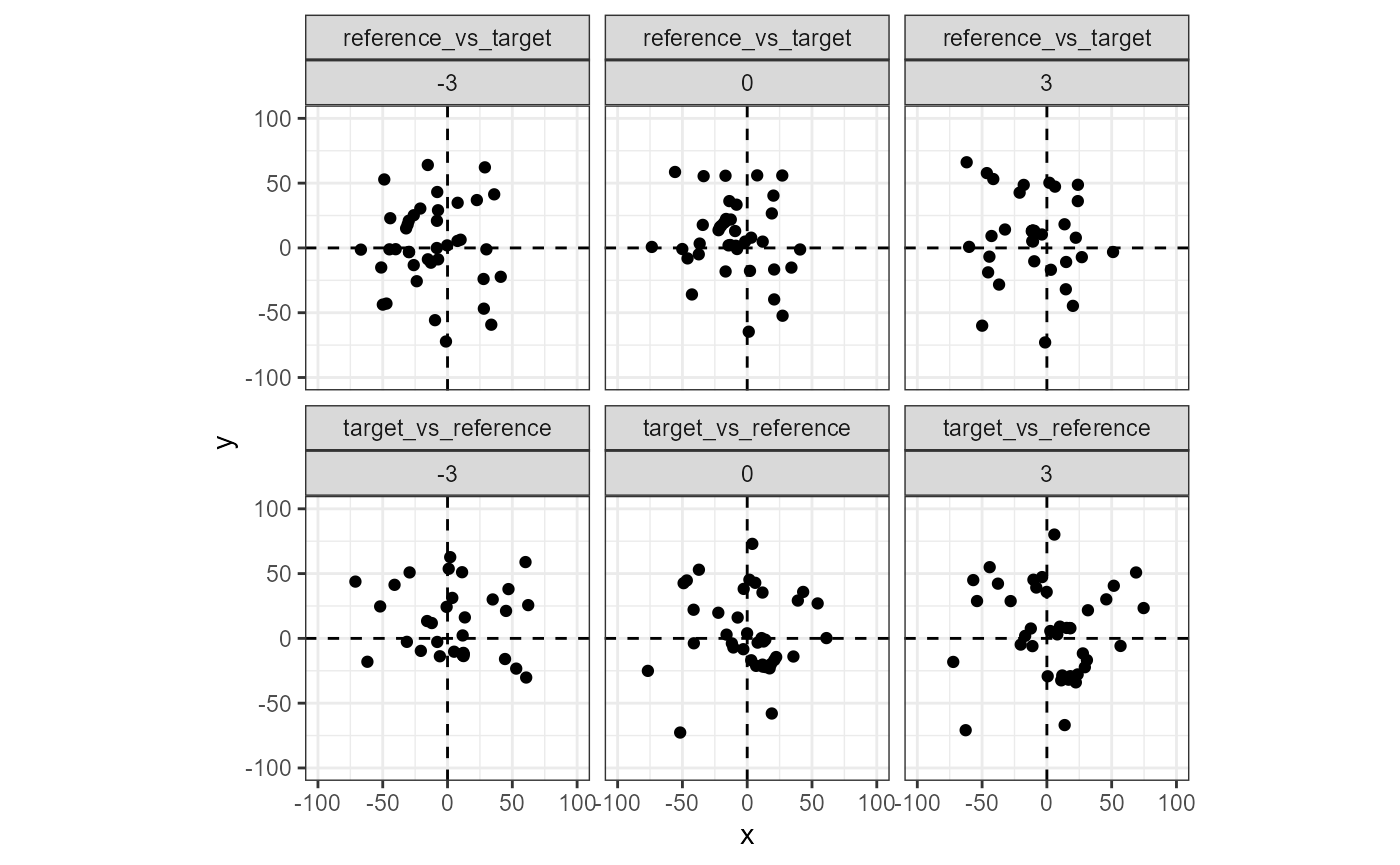
We can consider the notion of cell “agreement” through a different lens: considering just the estimated registration values, are there regions in rotation/translation, \((\theta, x, y)\), space where multiple cells seem to “bunch up?” The plot below shows the estimated translations per cell across three rotation angles, \(\{-3^\circ, 0^\circ, 3^\circ\}\), and both comparison directions. Note that the points in the “reference vs. target” direction appear to bunch-up around \(\theta = 3\) and \((x,y) = (-10,10)\). Conversely, the points in the “target vs. reference” direction bunch-up around \(\theta = 3\) and \((x,y) = (10,-10)\). This provides evidence that the scans are matching in two ways: (1) multiple cells in both directions “agree” on a particular rotation/translation and (2) the agreed-upon rotation/translation are opposites of each other between the two comparison directions.

comparisonData %>%
  filter(theta >= -3 & theta <= 3) %>%
  ggplot(aes(x=x,y=y)) +
  geom_jitter() +
  facet_wrap(direction~theta,nrow =  2) +
  xlim(c(-100,100)) +
  ylim(c(-100,100)) +
  coord_fixed() +
  theme_bw() +
  geom_vline(xintercept = 0,linetype = "dashed") +
  geom_hline(yintercept = 0,linetype = "dashed") 

The notion of “agreement” is formalized using the point density. The feature_densityBased_all function calculates three features related to the number of cells that agree upon a particular rotation/translation and whether the estimation rotations/translations are opposites of each other between the two comparison directions.

comparisonData %>%
  feature_densityBased_all(eps = 5,minPts = 5)
#> # A tibble: 1 × 4
#>   thetaDiff translationDiff clusterSize clusterInd
#>       <dbl>           <dbl>       <dbl> <lgl>     
#> 1         0            1.16          11 TRUE

Visual Diagnostic-based Features

comparisonDat_fullScan_estimRotation <- comparison_fullScan(K013sA1,K013sA2,
                                                            returnX3Ps = TRUE,
                                                            thetas = -3)

comparisonDat_fullScan_estimRotation %>%
  group_by(direction) %>%
  feature_visualDiagnostic_all()
#> # A tibble: 2 × 9
#>   direction      neigh…¹ neigh…² neigh…³ neigh…⁴ diffe…⁵ diffe…⁶ filte…⁷ filte…⁸
#>   <chr>            <dbl>   <dbl>   <dbl>   <dbl>   <dbl>   <dbl>   <dbl>   <dbl>
#> 1 reference_vs_…    74.4      NA    883.      NA -0.0344      NA    2.53      NA
#> 2 target_vs_ref…    97.4      NA    822.      NA  0.0858      NA    4.86      NA
#> # … with abbreviated variable names ¹​neighborhoodSizeAve_ave,
#> #   ²​neighborhoodSizeAve_sd, ³​neighborhoodSizeSD_ave, ⁴​neighborhoodSizeSD_sd,
#> #   ⁵​differenceCor_ave, ⁶​differenceCor_sd, ⁷​filteredRatio_ave,
#> #   ⁸​filteredRatio_sd